Examining the impact of an Accommodation and Support Intervention in reducing homelessness amongst Care Leavers in Australia: A hybrid type-1 Implementation-Effectiveness Study using Propensity Score methods — supplementary material
David Taylor 
Jessica Roberts
Aron Shlonsky
About
This page contains supplementary material for a study titled “Examining the impact of an Accommodation and Support Intervention in reducing homelessness amongst Care Leavers in Australia: A hybrid type-1 Implementation-Effectiveness Study using Propensity Score methods”.
The following information is provided here:
STROBE checklist — details of how this paper meets the STROBE reporting guidelines for observational studies.
Propensity Score Methods reporting checklist — details how this paper fulfils the guidelines on PSM reporting suggested by Thoemmes & Kim (2011).
Variables from administrative data — defines the variables used in our matching and outcome models.
Matching diagnostic tests — includes the diagnostic visualisations we used to assess covariate balance and common support.
Focus groups with intervention participants — provides details on participants, recruitment and consent procedures and protocols
Focus groups with provider and funder stakeholders — provides details on participants, consent procedures and protocols
Treatment effect results — includes the full results of our ATT estimates
Heterogenous treatment effects — includes figures depicting the results of our analysis of heterogenous treatment effects
Subgroup analysis — includes the full results of our subgroup analysis estimating conditional ATT by sex, Aboriginal status and housing vulnerability
Sensitivity analysis — includes results of our tipping point analysis for assess for the existence of unmeasured confounding
The code to produce this supplementary material, along with the analysis code for this review is available in a GitHub repository.
Reporting Standards
STROBE checklist
The STROBE checklist (Elm et al., 2007) with RECORD extension (Benchimol et al., 2015) is included in Table S1.
| Item No. | STROBE Items | Location in Manuscript | RECORD Items | Location in Manuscript |
|---|---|---|---|---|
| 1 | (a) Indicate the study’s design with a commonly used term in the title or the abstract (b) Provide in the abstract an informative and balanced summary of what was done and what was found |
(a) Use of propensity score methods are cited in the title (b) Details are provided in the abstract |
RECORD 1.1: The type of data used should be specified in the title or abstract. When possible, the name of the databases used should be included. RECORD 1.2: If applicable, the geographic region and timeframe within which the study took place should be reported in the title or abstract. RECORD 1.3: If linkage between databases was conducted for the study, this should be clearly stated in the title or abstract. |
1.1. This has been specified in the abstract 1.2. The country the study was undertaken in was specified in the title. The state was specified in the abstract 1.3. Specified in the abstract |
| 2 | Explain the scientific background and rationale for the investigation being reported | See Introduction | ||
| 3 | State specific objectives, including any prespecified hypotheses | See ‘Objectives’ section in the Introduction | ||
| 4 | Present key elements of study design early in the paper | See ‘Objectives’ section in the Introduction and Methodology | ||
| 5 | Describe the setting, locations, and relevant dates, including periods of recruitment, exposure, follow-up, and data collection | See ‘Intervention location’ and ‘Participants and recruitment’ sections in Methodology | ||
| 6 | (a) Cohort study - Give the eligibility criteria, and the sources and methods of selection of participants. Describe methods of follow-up (b) Cohort study - For matched studies, give matching criteria and number of exposed and unexposed |
(a) See section ‘Intervention inclusion and exclusion criteria’ (b) See ‘Identification and Estimation Strategy’ for criteria and Table 2 for counts |
RECORD 6.1: The methods of study population selection (such as codes or algorithms used to identify subjects) should be listed in detail. If this is not possible, an explanation should be provided. RECORD 6.2: Any validation studies of the codes or algorithms used to select the population should be referenced. If validation was conducted for this study and not published elsewhere, detailed methods and results should be provided. RECORD 6.3: If the study involved linkage of databases, consider use of a flow diagram or other graphical display to demonstrate the data linkage process, including the number of individuals with linked data at each stage. |
6.1. See section ‘Participants and recruitment’ 6.2. Not applicable for this study 6.3. See section ‘Data and Measures’ |
| 7 | Clearly define all outcomes, exposures, predictors, potential confounders, and effect modifiers. Give diagnostic criteria, if applicable. | See Table S3 | RECORD 7.1: A complete list of codes and algorithms used to classify exposures, outcomes, confounders, and effect modifiers should be provided. If these cannot be reported, an explanation should be provided. | 7.1. See ‘Identification and estimation strategy’ and specifically, the DAG in Figure 1 |
| 8 | For each variable of interest, give sources of data and details of methods of assessment (measurement). Describe comparability of assessment methods if there is more than one group | See ‘Data and measures’ section and Table S3 | ||
| 9 | Describe any efforts to address potential sources of bias | See ‘Identification and Estimation Strategy’ section and the DAG in Figure 1 | ||
| 10 | Explain how the study size was arrived at | See Table 2 for matching results and matched sample size | ||
| 11 | Explain how quantitative variables were handled in the analyses. If applicable, describe which groupings were chosen, and why | See section ‘Treatment Effect Estimation’ | ||
| 12 | (a) Describe all statistical methods, including those used to control for confounding (b) Describe any methods used to examine subgroups and interactions (c) Explain how missing data were addressed (d) Cohort study - If applicable, explain how loss to follow-up was addressed (e) Describe any sensitivity analyses |
(a) See ‘Propensity Score Matching Specification’ and ‘Treatment Effect Estimation’ (b) See ‘Treatment Effect Heterogeneity’ and ‘Subgroup Analysis’ sections (c) Not applicable (d) Not applicable (e) See ‘Sensitivity Analysis’ and section Section 4.5 |
RECORD 12.1: Authors should describe the extent to which the investigators had access to the database population used to create the study population. RECORD 12.2: Authors should provide information on the data cleaning methods used in the study. RECORD 12.3: State whether the study included person-level, institutional-level, or other data linkage across two or more databases. The methods of linkage and methods of linkage quality evaluation should be provided. |
12.1. See first paragraphs of Methodology 12.2. See section ‘Data and Measures’ 12.3. See section ‘Data and Measures’ |
| 13 | (a) Report the numbers of individuals at each stage of the study (e.g., numbers potentially eligible, examined for eligibility, confirmed eligible, included in the study, completing follow-up, and analysed) (b) Give reasons for non-participation at each stage. (c) Consider use of a flow diagram |
(a) See Table 2 for matching results and final analysis sample sizes (b) See section ‘Propensity Score Matching Specification’ (c) This is not appropriate for our study design |
RECORD 13.1: Describe in detail the selection of the persons included in the study (i.e., study population selection) including filtering based on data quality, data availability and linkage. The selection of included persons can be described in the text and/or by means of the study flow diagram. | 13.1 See sections ‘Participants and recruitment’; ‘Data and Measures’ and ‘Population characteristics’ |
Propensity Score Methods reporting checklist
The checklist of reporting guidelines by Thoemmes and Kim (2011) is detailed in Table S2.
| # | Characteristic | Location in manuscript |
|---|---|---|
| 1 | List of all covariates that were collected (with reliabilities) | Supplementary material Table S3 |
| 2 | List of all covariates that were used to estimate the propensity score | Supplementary material Figure S1 |
| 3 | Method that was used to determine set of covariates used for estimation (e.g., nonparsimonious model, predetermined significance threshold) | See section ‘Propensity Score Matching Specification’ |
| 4 | Inclusion of polynomial or interaction terms | Not applicable |
| 5 | Estimation method for propensity scores (e.g., logistic regression, regression trees) | See section ‘Propensity Score Matching Specification’ |
| 6 | Conditioning strategy (e.g., matching, stratification, weighting) | See section ‘Propensity Score Matching Specification’ |
| 7 | Region of common support (histograms, ranges) | Supplementary material Figure S2 |
| 8 | Details on matching scheme, if applicable | See section ‘Propensity Score Matching Specification’ |
| 8.1 | Type of matching algorithm (e.g., nearest neighbor, optimal, full, kernel) | See section ‘Propensity Score Matching Specification’ |
| 8.2 | Number of treated and control units that were matched with each other (e.g., 1:1, 1:many) | See section ‘Propensity Score Matching Specification’ |
| 8.3 | Matching with or without replacement | See section ‘Propensity Score Matching Specification’ |
| 8.4 | Caliper width, if applicable | Not applicable |
| 9 | Details on stratification, if applicable | Not applicable |
| 9.1 | Number of strata | Not applicable |
| 9.2 | Strategy to define strata (equal proportions, minimize variance) | Not applicable |
| 10 | Details on weighting, if applicable | Not applicable |
| 10.1 | Type of weights used (inverse probability weights, odd weights) | Not applicable |
| 10.2 | Distribution of weights, reporting of unusually large weights | Not applicable |
| 11 | Sample size before and after conditioning; report effective sample size if weights are used | This is included in Table 2 |
| 12 | Standardized difference before and after matching on the propensity score and all covariates, potentially also on interactions and quadratic terms | Supplementary material Figure S1 |
| 13 | Point estimate of treatment effect and associated standard error | This is summarised in Table 3 with additional detail provided in supplementary material: Table S8, Table S9 |
| 14 | Inclusion of covariates in outcome model | This is detailed in the section ‘Treatment Effect Estimation’ |
Supplementary methodology
Variables from administrative data
We have defined the variables that we used in our matching and outcome models in Table S3 below.
| Variable | Definition | Source |
|---|---|---|
male |
Binary indicator for male | ChildStory |
aboriginal |
Binary indicator for Aboriginal and Torres Strait Islander status ever recorded | ChildStory |
eligible_residential_care_placement |
Binary indicator for whether an individual was in a placement type recorded as “Residential Care” during their eligibility window | ChildStory |
eligible_time_in_care |
Binary indicator for whether an individual had spent 12 or more months in OOHC by either the start or end of their eligibility window | ChildStory |
eligible_placement_instability |
Binary indicator capturing placement instability through either: (1) More than 3 placements (lasting 30+ days) by either the start or end of eligibility window, OR (2) Any placement (lasting 30+ days) in either 6 months before eligibility window, 12 months before eligibility window, or during eligibility window itself, OR (3) Being in independent living arrangements in their last placement | ChildStory |
eligible_permanent_placement |
Binary indicator for whether an individual was in a placement with purpose recorded as “Permanent Care” during their eligibility window | ChildStory |
eligible_kinship_care_placement |
Binary indicator for whether an individual was in a kinship care placement during their eligibility window | ChildStory |
parental_responsibility_minister_eligiblity_period |
Binary indicator for whether the Minister had parental responsibility for the individual during their eligibility window | ChildStory |
any_housing_spell_before_18 |
Binary indicator for whether an individual had any contact with SHS for ‘housing reasons’ between their 16th and 18th birthday | CIMS |
in_housing_spell_on_date_18 |
Binary indicator for being in a SHS spell on their 18th birthday | CIMS |
in_housing_spell_on_date_19 |
Binary indicator for being in a SHS spell on their 19th birthday | CIMS |
new_housing_spell_between_18_19 |
Binary indicator for any new SHS spell between 18th and 19th birthday | CIMS |
new_ongoing_housing_spell_between_18_19 |
Binary indicator for either continuing or new SHS spell between 18th and 19th birthday | CIMS |
new_unsheltered_homelessness_between_18_19 |
Binary indicator for new spell of unsheltered homelessness between 18th and 19th birthday, where unsheltered homelessness is defined as either: (1) current residential dwelling is a tent, improvised dwelling, no dwelling (in the open), or motor vehicle, OR (2) residential dwelling in last week was a tent, improvised dwelling, no dwelling (in the open), or motor vehicle, OR (3) reported sleeping rough or in non-conventional accommodation in the last week | CIMS |
new_ongoing_unsheltered_homelessness_between_18_19 |
Binary indicator for a new or continuing spell of unsheltered homelessness between 18th and 19th birthday, where unsheltered homelessness is defined as either: (1) current residential dwelling is a tent, improvised dwelling, no dwelling (in the open), or motor vehicle, OR (2) residential dwelling in last week was a tent, improvised dwelling, no dwelling (in the open), or motor vehicle, OR (3) reported sleeping rough or in non-conventional accommodation in the last week | CIMS |
new_short_term_accommodation_required_between_18_19 |
Binary indicator for new spell requiring short-term accommodation between 18th and 19th birthday (based on Short_Term_Accom_ind in CIMS) | CIMS |
new_ongoing_short_term_accommodation_required_between_18_19 |
Binary indicator for either continuing or new spell requiring short-term accommodation between 18th and 19th birthday (based on Short_Term_Accom_ind in CIMS) | CIMS |
count_total_spells_18_19 |
Count of total number of distinct SHS spells between 18th and 19th birthday | CIMS |
time_in_housing_support_18_19 |
Total days in SHS between 18th and 19th birthday | CIMS |
Focus groups with intervention participants
Participant details
Focus groups with a sample of intervention participants were conducted face-to-face. Participants from all sites were represented. Details are summarised in Table S4.
| PYI provider catchment | Location of focus group | Number of attendees | Month held |
|---|---|---|---|
| Central Coast & Hunter | Newcastle | 12 | October 2019 |
| Mid North Coast & Northern NSW | Lismore | 8 | October 2019 |
| New England | Tamworth | <5 | October 2019 |
| Western NSW | Bathurst | <5 | October 2019 |
| South Western Sydney | Campbelltown | 6 | November 2019 |
| Nepean Blue Mountains | Penrith | 5 | November 2019 |
| Illawarra Shoalhaven & Southern NSW | Wollongong | <5 | November 2019 |
Recruitment and consent process
Invitation
- The Evaluation Team contacted providers by email in September 2019 and requested their assistance to identify and approach clients who might be willing to participate in a focus group to discuss PYI
- Additional contact was made with provider contacts to answer questions and clarify the content and scope of the focus group
Recruitment
- Young people receiving PYI services, aged 18 years or older, were invited by their PYI providers to participate in a focus group on the PYI program (PYI providers were provided with an explanatory statement, consent forms and protocol to assist in the recruitment of young people for interview)
- Providers used the Explanatory Statement approved by the Monash University Human Research Ethics Committee to inform young people about the purpose and nature of the focus group and invite them to participate
Focus groups
- Focus groups were held in-person at or near the PYI providers usual place of business
- Sessions lasted for between 60 minutes
- Sessions were facilitated by two experienced qualitative researchers from CEI — one of whom had qualifications in either social work or psychology — who shared roles as moderator and scribe
- A semi-structured protocol was developed to guide discussion — it is included in Section 3.2.3.
Consent
- Prior to the focus group participants were provided with a copy of the Explanatory Statement, consent details and focus group protocol
- The facilitator verbally went through the explanatory statement and consent procedures prior to commencement
- Participants signed a consent form with one copy retained by the participant and one retained by the facilitator
- Young people who provided consent to participate in the focus groups were provided with a gift voucher — not redeemable for alcohol or tobacco products — valued at $25
- Respondent feedback was recorded by hand by facilitators anonymously to protect the confidentiality of respondents
Focus group protocol
Introduction
- How long have you been involved in PYI services?
Personal advisor
- Do you all have a personal advisor?
- Did your personal advisor help you by:
- supporting you to complete your leaving care plan?
- assisting you to grow your support network?
- Is there anything they could have done differently?
Transitional support
- Have you all met with your transitional support worker?
- Did your transitional support worker help you by:
- asking about your accommodation needs?
- assisting with securing accommodation by working with a real estate agent or community housing provider?
- Is there anything they could have done differently?
Education and employment mentoring
- Have you all met with your education and employment mentor?
- How did they help you?
- Did they help you by:
- Choosing education and employment goals?
- Helping you apply for education / jobs?
- Is there anything they could have done differently?
General feedback
- Were you able to get help when you needed it?
- Would you like to add anything about stuff that’s been challenging for you, that you would like to see improved with PYI?
- Is there anything about stuff that you really enjoy about PYI that you would like to see more of?
Overall
- Do you have any other feedback on how PYI could be improved?
Focus groups with representatives from service and housing providers
Participant details
PYI service providers
Focus groups were conducted in person with key representatives from PYI service providers. Participants across all sites included senior staff responsible for program management and funder engagement, as well as frontline workers who directly supported program participants. Representatives from all service providers participated in the focus groups. Details of the focus group composition and locations are summarised in Table S5.
| PYI provider catchment | Location of focus group | Number of attendees | Month held |
|---|---|---|---|
| Central Coast & Hunter | Newcastle | 10 | October 2019 |
| Mid North Coast & Northern NSW | Lismore | 5 | October 2019 |
| New England | Tamworth | <5 | October 2019 |
| Western NSW | Bathurst | <5 | October 2019 |
| South Western Sydney | Campbelltown | 5 | November 2019 |
| Nepean Blue Mountains | Penrith | 5 | November 2019 |
| Illawarra Shoalhaven & Southern NSW | Wollongong | <5 | November 2019 |
PYI housing providers
Housing provision for participants was managed either through a dedicated role within the service provider organisation or by a separate organization for those operating within a consortium. Interviews with housing provider representatives were conducted independently from service provider interviews due to their distinct focus. These interviews were conducted virtually via Zoom due to COVID-19 social distancing restrictions in place at the time. All housing providers except one participated in the interviews. Details of the interviews are summarised in Table Table S6.
| PYI provider catchment | Month held |
|---|---|
| Central Coast & Hunter | August 2020 |
| Mid North Coast & Northern NSW | August 2020 |
| New England | August 2020 |
| South Western Sydney | August 2020 |
| Nepean Blue Mountains | Not held |
| Illawarra Shoalhaven & Southern NSW | August 2020 |
Recruitment and consent process
Invitation:
- The Evaluation Team contacted PYI providers by email in August and September 2019 to provide information about the focus groups and their scope.
- The Evaluation Team contacted PYI housing providers by email in August 2020 to provide information about the focus groups and their scope.
- Additional contact was made with provider contacts to answer questions and clarify the content and scope of the focus groups.
Recruitment:
- Providers were emailed a copy of the Explanatory Statement and focus group protocol approved by the Monash University Human Research Ethics Committee and asked to review it and identify the individuals within their organisation who were best placed to provide input.
- The Evaluation Team liaised with providers to find a mutually beneficial date and time to hold the focus group.
Consent:
- Prior to the focus group participants were provided with a copy of the Explanatory Statement, consent details and protocol
- The facilitator verbally went through the explanatory statement and consent procedures prior to commencement
Focus group protocol
We have developed a protocol based upon the domains of the Consolidated Framework for Implementation Research (CFIR). The CFIR is a meta-theoretical framework that synthesises information and evidence about constructs and domains that affect implementation processes.
Implementation enablers and barriers can be related to five different areas: the types of services offered; the individuals involved in implementing the service; the organisation setting in which the service is implemented; the organisations outer context; and the quality of the implementation process itself. In the focus group, we will briefly discuss the five areas that impact implementation and then ask for your input about which areas you think are key challenges or enablers for PYI service providers.
Note: This discussion guide is indicative and may not be reflective of the exact content
Purpose and consent
Evaluation Team to provide brief overview of the purpose of the focus group and how it will be used to inform the evaluation. Verbal consent will be obtained in order to record the teleconference and use the information provided to inform our evaluation findings.
Introductions
Please introduce yourself to the group and tell us how long you have been involved with the Premiers Youth Initiative (PYI). What is your current role (program manager, executive manager, administrator) in relation to PYI?
The types of services offered
What is it? — The types of services offered are important because the different attributes (complexity, adaptability, cost, evidence strength and quality and design quality) of the services will influence how easy it can be taken up by individuals and service provider agencies.
Indicative talking points:
- What are some troubles that your clients face?
- What do you do to help clients?
- Is there anything you can’t do?
The Individuals involved
What is it? — The individuals involved in implementing the service are important because their skills, expertise, attitudes, behaviours and values influence how they engage in the implementation process and how the organisation setting operates.
Indicative talking points:
- How were the PYI guidelines interpreted by your team?
- What are they three things that they do always?
- How do they work together?
The external context
What is it? — The organisation’s outer context is important because funding structures, legislation, policy agendas and similar factors in the environment of the implementation can change or totally stop an implementation.
Indicative talking points:
- What challenges did you experience outside of your workplace (i.e. outside your control) that have made it difficult to implement PYI?
- Are you able to get the things they need in a timely fashion?
- Are there things that they need that you can’t get them?
The organisational context
What is it? — The organisation setting in which the service is implemented is important because factors such as hierarchical structures, culture, communication and access to training and resources will influence how quickly and easily a new program can be taken up and utilised by an organisation.
Indicative talking points:
- In what ways were service providers well-prepared to deliver PYI?
- How do you know what your clients need?
The quality of the implementation process
What is it? — The quality of the implementation process itself is important because the attention paid, resources invested, and commitment made to an implementation process will enhance, or diminish, the likelihood of its success.
Indicative talking points:
- How did the process of implementing the PYI work?
- What are you doing that works to improve outcomes for your clients?
Overall
Do you have any other feedback on how PYI could be strengthened to better meet the needs of the young people it seeks to support? Please explain.
Focus groups with representatives from the funder
Participant details
The intervention was developed and funded by the NSW Department of Communities and Justice (DCJ). Program oversight was managed by the central office in Sydney, while day-to-day engagement between the funding body and service providers was coordinated by district-level representatives. Focus group participants included the program manager (from the central office) and contract managers from all districts where the intervention was implemented. These focus groups were conducted virtually via Zoom due to COVID-19 social distancing restrictions in place at the time. Details are summarised in Table S7.
| PYI provider catchment | Number of attendees | Month held |
|---|---|---|
| Statewide — Central office | 3 | August 2020 |
| Central Coast, Hunter & New England | 4 | August 2020 |
| Mid North Coast & Northern NSW | 2 | August 2020 |
| Western NSW, Illawarra Shoalhaven & Southern NSW | 2 | August 2020 |
| South Western Sydney & Nepean Blue Mountains | 4 | August 2020 |
Recruitment and consent process
Invitation:
- Representatives from the funder were nominated by the program manager at DCJ central office.
- The Evaluation Team contacted nominated contacts by email in August 2020 to provide information about the focus groups and their scope.
Recruitment:
- Nominated representatives from DCJ were emailed a copy of the Explanatory Statement and protocol approved by the Monash University Human Research Ethics Committee and asked to review it prior to the focus group.
- The Evaluation Team liaised with representatives from DCJ to find a mutually beneficial date and time to hold the focus group.
Consent:
- The facilitator verbally went through the explanatory statement and consent procedures prior to commencement
Protocol
We have compiled a series of questions based upon the domains of the Consolidated Framework for Implementation Research (CFIR). The CFIR is a meta-theoretical framework that synthesises information and evidence about constructs and domains that affect implementation processes.
Implementation enablers and barriers can be related to five different areas: the types of services offered; the individuals involved in implementing the service; the organisational setting in which the service is implemented; the organisations outer context; and the quality of the implementation process itself. We are interested in obtaining your input about which areas you think are key challenges or enablers in the implementation of PYI.
Note: This discussion guide is indicative and may not be reflective of the exact content
The types of services offered
What is it? — The types of services offered are important because the different attributes (complexity, adaptability, cost, evidence strength and quality and design quality) of the services will influence how easy it can be taken up by individuals and service provider agencies.
Specific questions:
- In what context was PYI developed?
- How was this population served before PYI? • How did it fit into the broader policy/reform context?
- What decisions led to the current model being pursued?
The Individuals involved
What is it? — The individuals involved in implementing the service are important because their skills, expertise, attitudes, behaviours and values influence how they engage in the implementation process and how the organisation setting operates.
Specific questions:
- How were the program’s goals decided?
- How was local demand for services estimated in each location?
The external context
What is it? — The organisation’s outer context is important because funding structures, legislation, policy agendas and similar factors in the environment of the implementation can change or totally stop an implementation.
Specific questions:
- By the time they left care, what did DCJ envision PYI clients would be prepared for by their case workers?
The organisational context
What is it? — The organisation setting in which the service is implemented is important because factors such as hierarchical structures, culture, communication and access to training and resources will influence how quickly and easily a new program can be taken up and utilised by an organisation.
Specific questions:
- What does a successful outcome for PYI clients look like from DCJ’s perspective?
The quality of the implementation process
What is it? — The quality of the implementation process itself is important because the attention paid, resources invested, and commitment made to an implementation process will enhance, or diminish, the likelihood of its success.
Specific questions:
- Did you think the CIT and DIT structure suited the needs of this project?
- What elements of this structure/process do you think worked well?
Overall
- Do you have any thoughts on how PYI could be strengthened to better meet the needs of the young people it seeks to support? Please explain.
Supplementary results
Matching diagnostic tests
Assessing sample balance
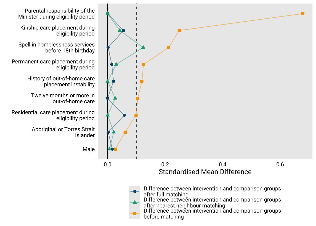
Figure S1 presents a love plot, a diagnostic tool for assessing covariate balance before and after matching. It displays the standardized mean differences (SMDs) for each covariate included in the matching model, providing a scale-independent measure of balance that is unaffected by sample size. Covariate balance is essential for causal inference, as it ensures that intervention and comparison groups are sufficiently comparable, reducing sensitivity to model misspecification and improving the validity of treatment effect estimates. Prior to matching, six of nine covariates exceeded the commonly recommended threshold of 0.1 SMD, indicating poor balance; however, both matching methods improved balance substantially, with full matching achieving excellent balance across all covariates.
Assessing common support
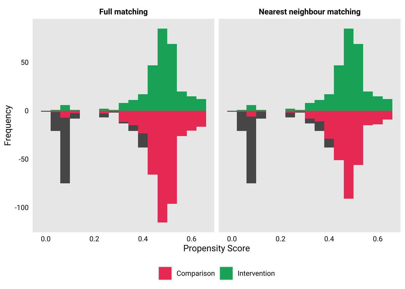
The common support assumption requires that the probability of receiving treatment conditional on covariates \(X\) lies strictly between 0 and 1: \(0 < P(D=1|X) < 1\) where \(D\) is the treatment indicator and \(X\) represents the vector of covariates used for matching. This condition requires that there is overlap in the distribution of propensity scores between those who receive the intervention and comparison across the range of scores, in order for a counterfactual to be valid (Heckman, Ichimura, & Todd, 1997). We assessed this visually using a balance plot (Figure S2), which shows the distribution of propensity scores for the intervention and comparison groups under both matching specifications. The plot shows that both specifications achieve substantial overlap in the propensity score distributions between individuals in the intervention and comparison samples, suggesting the analysis meets the common support assumption.
Treatment effect results
| In homelessness spell on 18th birthday | In homelessness spell on 19th birthday | New homelessness spell between 18th & 19th birthday | New or ongoing homelessness spell between 18th & 19th birthday | New unsheltered homelessness spell between 18th and 19th birthday | New or ongoing unsheltered homelessness spell between 18th and 19th birthday | In new homelessness spell that requires housing assistance between 18th & 19th birthday | In new or ongoing homelessness spell that requires short term accommodation between 18th & 19th birthday | Number of distinct homelessness spells between 18th and 19th birthday | Days in homelessness spell between 18th and 19th birthday | |
|---|---|---|---|---|---|---|---|---|---|---|
| Model family: | Quasibinomial | Quasibinomial | Quasibinomial | Quasibinomial | Quasibinomial | Quasibinomial | Quasibinomial | Quasibinomial | Poisson | Linear |
| Link function: | Logit | Logit | Logit | Logit | Logit | Logit | Logit | Logit | Log | Identity |
| Intervention group | 0.047 | 0.064 | 0.142 | 0.169 | 0.129 | 0.153 | 0.142 | 0.169 | 0.227 | 15.427 |
| Comparison group | 0.067 | 0.051 | 0.142 | 0.18 | 0.134 | 0.173 | 0.142 | 0.18 | 0.351 | 18.725 |
| ATT estimate | -0.02 | 0.013 | 0 | -0.011 | -0.006 | -0.02 | 0 | -0.011 | ||
| Standard error | (0.022) | (0.022) | (0.03) | (0.034) | (0.031) | (0.035) | (0.03) | (0.034) | ||
| 95% CI | [-0.068, 0.019] | [-0.032, 0.055] | [-0.06, 0.055] | [-0.076, 0.056] | [-0.074, 0.049] | [-0.09, 0.046] | [-0.06, 0.055] | [-0.076, 0.056] | ||
| ATT estimate | 0.709 | 1.255 | 1.003 | 0.94 | 0.958 | 0.882 | 1.003 | 0.94 | ||
| Standard error | (0.321) | (0.662) | (0.228) | (0.192) | (0.249) | (0.202) | (0.228) | (0.192) | ||
| 95% CI | [0.339, 1.481] | [0.584, 2.696] | [0.669, 1.503] | [0.645, 1.369] | [0.604, 1.518] | [0.58, 1.342] | [0.669, 1.503] | [0.645, 1.369] | ||
| ATT estimate | 0.694 | 1.272 | 1.004 | 0.927 | 0.952 | 0.86 | 1.004 | 0.927 | ||
| Standard error | (0.337) | (0.717) | (0.268) | (0.232) | (0.288) | (0.238) | (0.268) | (0.232) | ||
| 95% CI | [0.289, 1.545] | [0.543, 3.05] | [0.617, 1.624] | [0.596, 1.5] | [0.535, 1.59] | [0.521, 1.443] | [0.617, 1.624] | [0.596, 1.5] | ||
| ATT estimate | -0.124 | -3.298 | ||||||||
| Standard error | (0.079) | (4.931) | ||||||||
| 95% CI | [-0.279, 0.031] | [-12.963, 6.368] | ||||||||
| ATT estimate | -0.201 | 0.133 | 0.002 | -0.042 | -0.027 | -0.083 | 0.002 | -0.042 | -0.152 | -0.152 |
| Standard error | (0.231) | (0.24) | (0.137) | (0.131) | (0.154) | (0.144) | (0.137) | (0.131) | (0.086) | (0.086) |
| 95% CI | [-0.685, 0.238] | [-0.336, 0.615] | [-0.266, 0.268] | [-0.285, 0.223] | [-0.345, 0.256] | [-0.362, 0.202] | [-0.266, 0.268] | [-0.285, 0.223] | [-0.317, 0.014] | [-0.315, 0.013] |
| Number of Observations | 701 | 701 | 701 | 701 | 701 | 701 | 701 | 701 | 701 | 701 |
| In homelessness spell on 18th birthday | In homelessness spell on 19th birthday | New homelessness spell between 18th & 19th birthday | New or ongoing homelessness spell between 18th & 19th birthday | New unsheltered homelessness spell between 18th and 19th birthday | New or ongoing unsheltered homelessness spell between 18th and 19th birthday | In new homelessness spell that requires housing assistance between 18th & 19th birthday | In new or ongoing homelessness spell that requires short term accommodation between 18th & 19th birthday | Number of distinct homelessness spells between 18th and 19th birthday | Days in homelessness spell between 18th and 19th birthday | |
|---|---|---|---|---|---|---|---|---|---|---|
| Model family: | Quasibinomial | Quasibinomial | Quasibinomial | Quasibinomial | Quasibinomial | Quasibinomial | Quasibinomial | Quasibinomial | Poisson | Linear |
| Link function: | Logit | Logit | Logit | Logit | Logit | Logit | Logit | Logit | Log | Identity |
| Intervention group | 0.047 | 0.064 | 0.142 | 0.169 | 0.129 | 0.153 | 0.142 | 0.169 | 0.227 | 15.427 |
| Comparison group | 0.062 | 0.048 | 0.128 | 0.169 | 0.121 | 0.161 | 0.128 | 0.169 | 0.307 | 19.667 |
| ATT estimate | -0.014 | 0.016 | 0.014 | 0 | 0.008 | -0.008 | 0.014 | 0 | ||
| Standard error | (0.017) | (0.018) | (0.027) | (0.029) | (0.026) | (0.028) | (0.027) | (0.029) | ||
| 95% CI | [-0.049, 0.019] | [-0.02, 0.053] | [-0.038, 0.068] | [-0.057, 0.057] | [-0.043, 0.061] | [-0.063, 0.047] | [-0.038, 0.068] | [-0.057, 0.057] | ||
| ATT estimate | 0.769 | 1.34 | 1.112 | 1.002 | 1.062 | 0.948 | 1.112 | 1.002 | ||
| Standard error | (0.276) | (0.548) | (0.239) | (0.179) | (0.243) | (0.18) | (0.239) | (0.179) | ||
| 95% CI | [0.411, 1.438] | [0.705, 2.549] | [0.751, 1.646] | [0.717, 1.401] | [0.703, 1.604] | [0.667, 1.349] | [0.751, 1.646] | [0.717, 1.401] | ||
| ATT estimate | 0.757 | 1.364 | 1.13 | 1.003 | 1.071 | 0.939 | 1.13 | 1.003 | ||
| Standard error | (0.289) | (0.593) | (0.283) | (0.217) | (0.282) | (0.213) | (0.283) | (0.217) | ||
| 95% CI | [0.374, 1.493] | [0.669, 2.887] | [0.719, 1.815] | [0.665, 1.509] | [0.666, 1.769] | [0.612, 1.435] | [0.719, 1.815] | [0.665, 1.509] | ||
| ATT estimate | -0.08 | -4.24 | ||||||||
| Standard error | (0.059) | (4.458) | ||||||||
| 95% CI | [-0.196, 0.036] | [-12.979, 4.498] | ||||||||
| ATT estimate | -0.153 | 0.171 | 0.068 | 0.002 | 0.038 | -0.035 | 0.068 | 0.002 | -0.106 | -0.071 |
| Standard error | (0.193) | (0.205) | (0.13) | (0.114) | (0.136) | (0.12) | (0.13) | (0.114) | (0.082) | (0.082) |
| 95% CI | [-0.541, 0.222] | [-0.219, 0.588] | [-0.181, 0.329] | [-0.225, 0.227] | [-0.224, 0.315] | [-0.271, 0.199] | [-0.181, 0.329] | [-0.225, 0.227] | [-0.268, 0.055] | [-0.232, 0.091] |
| Number of Observations | 590 | 590 | 590 | 590 | 590 | 590 | 590 | 590 | 590 | 590 |
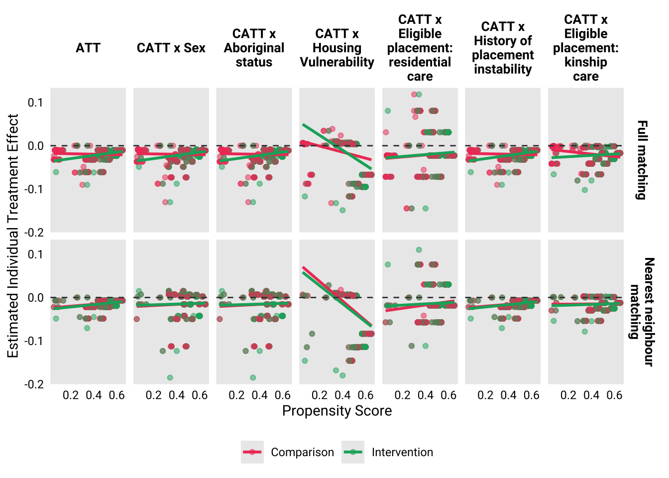
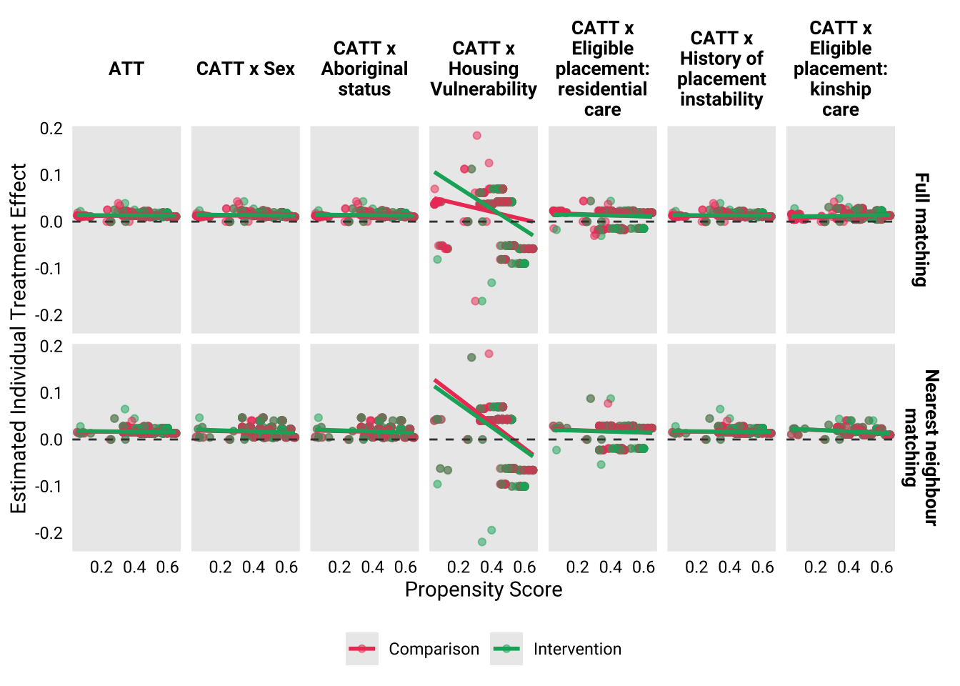
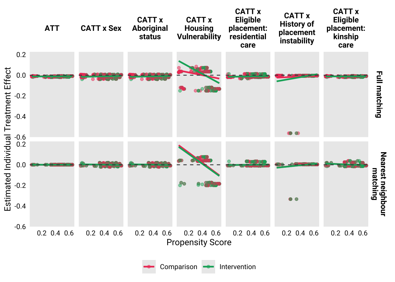
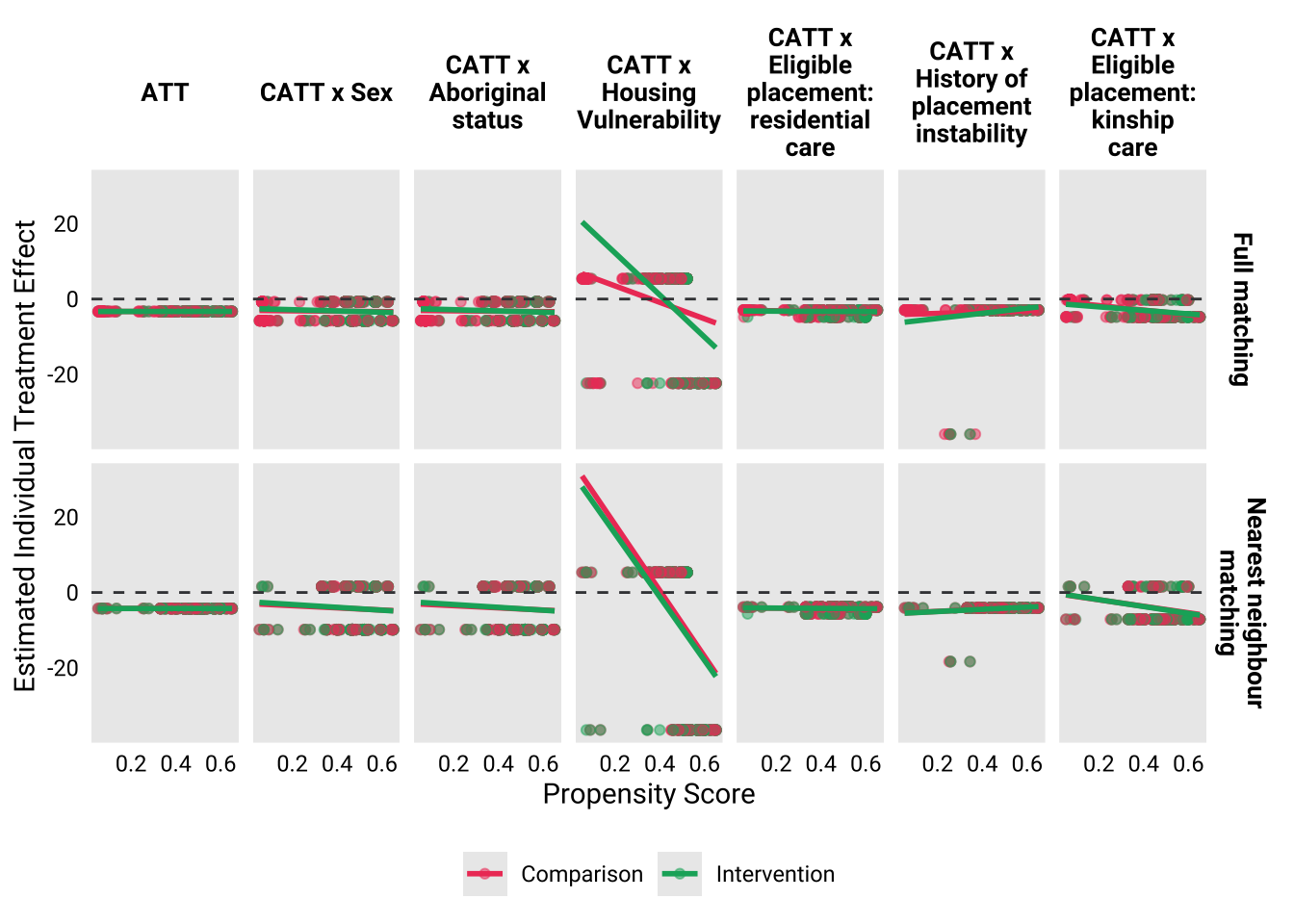
Heterogeneous treatment effects
HTE x ‘In homelessness spell on 18th birthday’
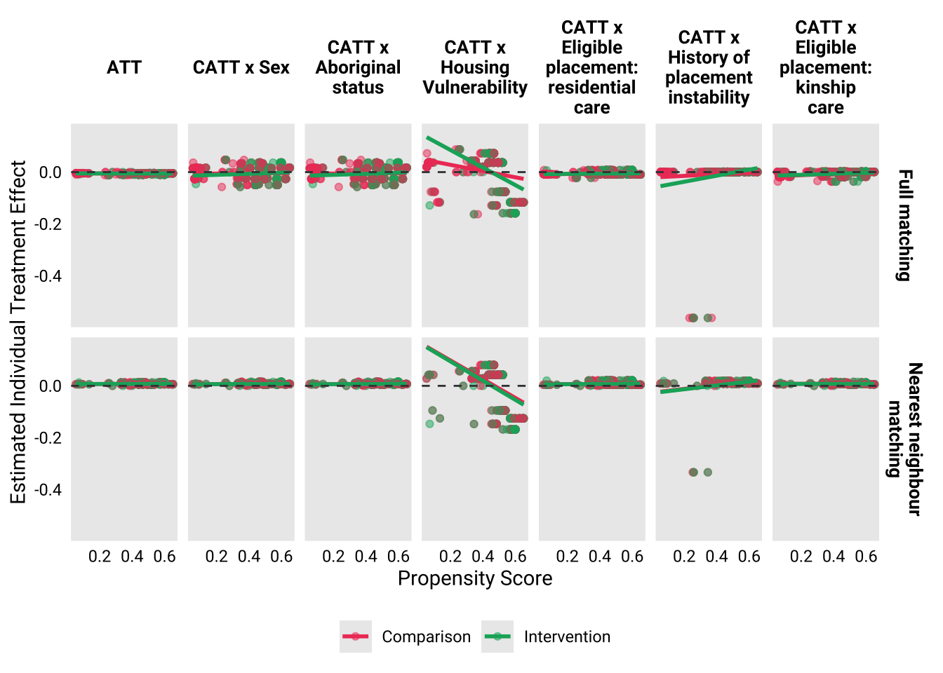
HTE x ‘In homelessness spell on 19th birthday’
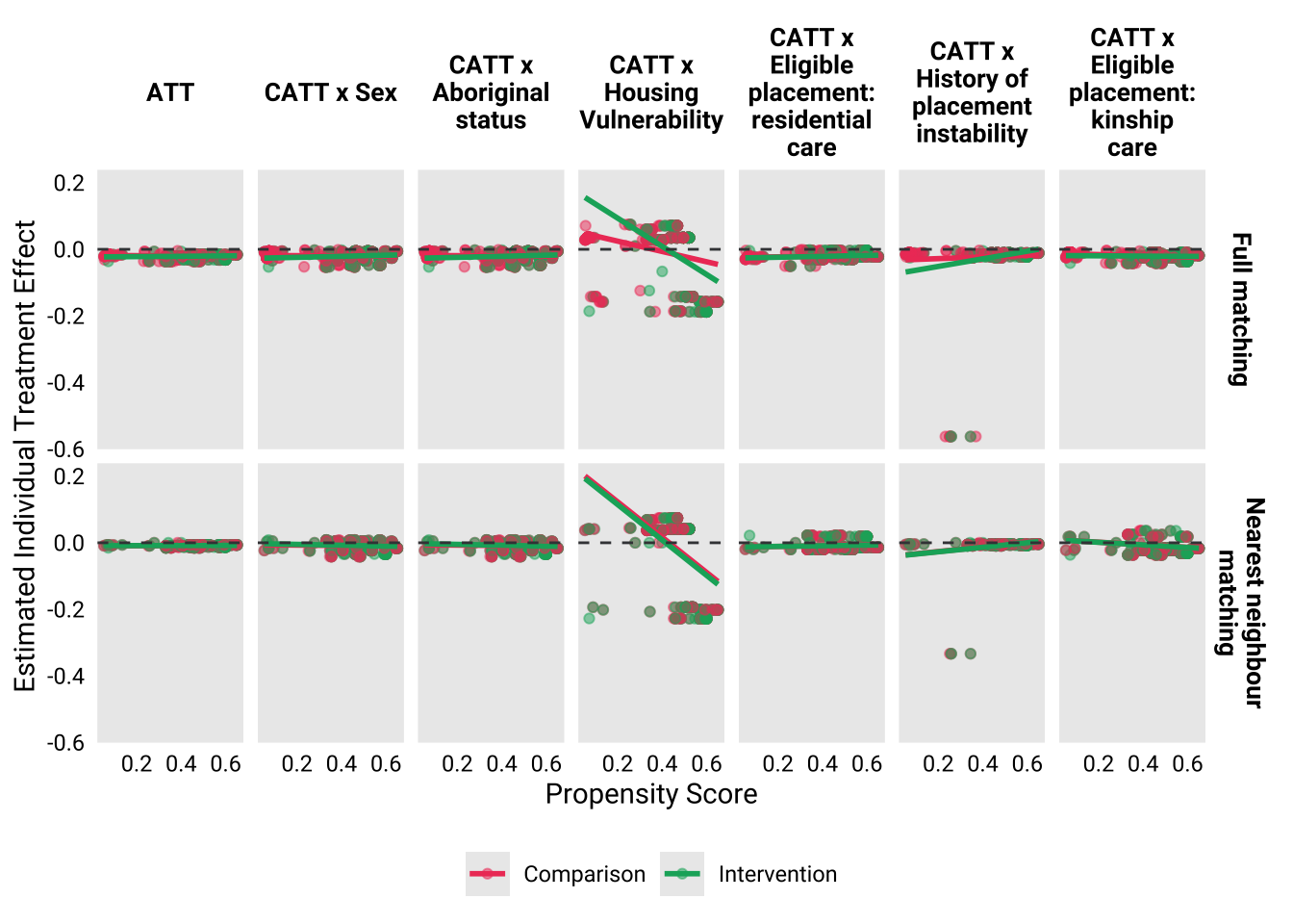
HTE x ‘New homelessness spell between 18th & 19th birthday’

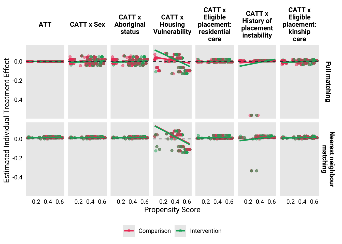
HTE x ‘New or ongoing homelessness spell between 18th & 19th birthday’
HTE x ‘New unsheltered homelessness spell between 18th and 19th birthday’
HTE x ‘New or ongoing unsheltered homelessness spell between 18th and 19th birthday’
HTE x ‘In new homelessness spell that requires short term accommodation between 18th & 19th birthday’
HTE x ‘In new or ongoing homelessness spell that requires short term accommodation between 18th & 19th birthday’

HTE x ‘Number of distinct homelessness spells between 18th and 19th birthday’
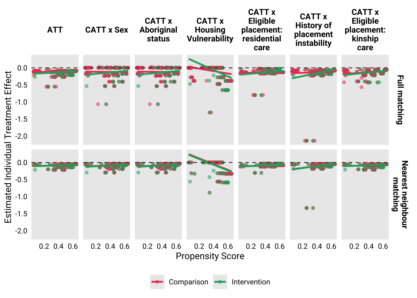
HTE x ‘Days in homelessness spell between 18th and 19th birthday’
Subgroup analysis
Subgroup analysis by sex
| In homelessness spell on 18th birthday | In homelessness spell on 19th birthday | New homelessness spell between 18th & 19th birthday | Any homelessness spell between 18th & 19th birthday | New unsheltered homelessness spell between 18th and 19th birthday | New or ongoing unsheltered homelessness spell between 18th and 19th birthday | In new homelessness spell that requires short term accommodation between 18th & 19th birthday | In new or ongoing homelessness spell that requires short term accommodation between 18th & 19th birthday | Number of distinct homelessness spells between 18th and 19th birthday | Days in homelessness spell between 18th and 19th birthday | |||||||||||
|---|---|---|---|---|---|---|---|---|---|---|---|---|---|---|---|---|---|---|---|---|
| Model family: | Binomial (MPL Jeffreys bias-reduced) | Binomial (MPL Jeffreys bias-reduced) | Binomial (MPL Jeffreys bias-reduced) | Binomial (MPL Jeffreys bias-reduced) | Binomial (MPL Jeffreys bias-reduced) | Binomial (MPL Jeffreys bias-reduced) | Binomial (MPL Jeffreys bias-reduced) | Binomial (MPL Jeffreys bias-reduced) | Poisson | Linear | ||||||||||
| Link function: | Logit | Logit | Logit | Logit | Logit | Logit | Logit | Logit | Log | Identity | ||||||||||
| Male | Female | Male | Female | Male | Female | Male | Female | Male | Female | Male | Female | Male | Female | Male | Female | Male | Female | Male | Female | |
| Intervention group | 0.065 | 0.036 | 0.079 | 0.056 | 0.161 | 0.129 | 0.195 | 0.149 | 0.147 | 0.116 | 0.182 | 0.129 | 0.161 | 0.129 | 0.195 | 0.149 | 0.262 | 0.193 | 18.228 | 12.72 |
| Comparison group | 0.077 | 0.056 | 0.063 | 0.042 | 0.182 | 0.099 | 0.216 | 0.14 | 0.175 | 0.092 | 0.209 | 0.133 | 0.182 | 0.099 | 0.216 | 0.14 | 0.507 | 0.185 | 18.487 | 17.662 |
| CATT estimate | -0.012 | -0.019 | 0.016 | 0.015 | -0.021 | 0.03 | -0.021 | 0.009 | -0.028 | 0.024 | -0.027 | -0.004 | -0.021 | 0.03 | -0.021 | 0.009 | ||||
| Standard error | (0.037) | (0.023) | (0.036) | (0.024) | (0.045) | (0.036) | (0.052) | (0.041) | (0.05) | (0.034) | (0.056) | (0.04) | (0.045) | (0.036) | (0.052) | (0.041) | ||||
| 95% CI | [-0.102, 0.047] | [-0.068, 0.025] | [-0.063, 0.078] | [-0.031, 0.062] | [-0.114, 0.063] | [-0.043, 0.099] | [-0.119, 0.083] | [-0.078, 0.087] | [-0.137, 0.063] | [-0.046, 0.091] | [-0.139, 0.078] | [-0.085, 0.072] | [-0.114, 0.063] | [-0.043, 0.099] | [-0.119, 0.083] | [-0.078, 0.087] | ||||
| CATT estimate | 0.848 | 0.652 | 1.246 | 1.347 | 0.884 | 1.305 | 0.905 | 1.064 | 0.842 | 1.256 | 0.87 | 0.969 | 0.884 | 1.305 | 0.905 | 1.064 | ||||
| Standard error | (0.737) | (0.444) | (1.262) | (1.165) | (0.265) | (0.48) | (0.252) | (0.333) | (0.302) | (0.482) | (0.278) | (0.319) | (0.265) | (0.48) | (0.252) | (0.333) | ||||
| 95% CI | [0.27, 2.417] | [0.19, 1.903] | [0.379, 3.776] | [0.44, 3.903] | [0.52, 1.545] | [0.665, 2.476] | [0.567, 1.554] | [0.577, 1.872] | [0.443, 1.563] | [0.621, 2.472] | [0.494, 1.562] | [0.512, 1.763] | [0.52, 1.545] | [0.665, 2.476] | [0.567, 1.554] | [0.577, 1.872] | ||||
| CATT estimate | 0.838 | 0.639 | 1.267 | 1.368 | 0.862 | 1.35 | 0.882 | 1.075 | 0.815 | 1.29 | 0.842 | 0.964 | 0.862 | 1.35 | 0.882 | 1.075 | ||||
| Standard error | (0.794) | (0.462) | (1.386) | (1.253) | (0.317) | (0.565) | (0.316) | (0.399) | (0.356) | (0.559) | (0.343) | (0.371) | (0.317) | (0.565) | (0.316) | (0.399) | ||||
| 95% CI | [0.247, 2.548] | [0.179, 1.956] | [0.351, 4.117] | [0.428, 4.127] | [0.456, 1.666] | [0.636, 2.766] | [0.491, 1.73] | [0.528, 2.066] | [0.377, 1.692] | [0.592, 2.717] | [0.415, 1.725] | [0.463, 1.907] | [0.456, 1.666] | [0.636, 2.766] | [0.491, 1.73] | [0.528, 2.066] | ||||
| CATT estimate | -0.245 | 0.009 | -0.26 | -4.942 | ||||||||||||||||
| Standard error | (0.146) | (0.059) | (7.557) | (6.174) | ||||||||||||||||
| 95% CI | [-0.532, 0.042] | [-0.108, 0.125] | [-15.071, 14.551] | [-17.043, 7.158] | ||||||||||||||||
| CATT estimate | -0.098 | -0.247 | 0.131 | 0.173 | -0.082 | 0.165 | -0.069 | 0.04 | -0.113 | 0.14 | -0.095 | -0.02 | -0.082 | 0.165 | -0.069 | 0.04 | -0.529 | 0.021 | -0.006 | -0.15 |
| Standard error | (0.332) | (0.333) | (0.339) | (0.314) | (0.18) | (0.205) | (0.178) | (0.189) | (0.21) | (0.21) | (0.201) | (0.197) | (0.18) | (0.205) | (0.178) | (0.189) | (0.365) | (0.162) | (0.212) | (0.245) |
| 95% CI | [-0.781, 0.509] | [-0.932, 0.386] | [-0.574, 0.787] | [-0.459, 0.793] | [-0.433, 0.281] | [-0.249, 0.562] | [-0.393, 0.301] | [-0.352, 0.4] | [-0.538, 0.29] | [-0.288, 0.553] | [-0.487, 0.296] | [-0.422, 0.356] | [-0.433, 0.281] | [-0.249, 0.562] | [-0.393, 0.301] | [-0.352, 0.4] | [-1.445, 0.015] | [-0.396, 0.249] | [-0.489, 0.288] | [-0.734, 0.177] |
| Difference | -0.008 | -0.008 | -0.001 | -0.001 | 0.051 | 0.051 | 0.03 | 0.03 | 0.051 | 0.051 | 0.023 | 0.023 | 0.051 | 0.051 | 0.03 | 0.03 | 0.254 | 0.254 | -4.683 | -4.683 |
| Standard error | (0.044) | (0.044) | (0.043) | (0.043) | (0.058) | (0.058) | (0.067) | (0.067) | (0.061) | (0.061) | (0.07) | (0.07) | (0.058) | (0.058) | (0.067) | (0.067) | (0.157) | (0.157) | (9.717) | (9.717) |
| 95% CI | [-0.094, 0.079] | [-0.094, 0.079] | [-0.086, 0.084] | [-0.086, 0.084] | [-0.063, 0.165] | [-0.063, 0.165] | [-0.101, 0.161] | [-0.101, 0.161] | [-0.069, 0.171] | [-0.069, 0.171] | [-0.114, 0.16] | [-0.114, 0.16] | [-0.063, 0.165] | [-0.063, 0.165] | [-0.101, 0.161] | [-0.101, 0.161] | [-0.054, 0.562] | [-0.054, 0.562] | [-23.727, 14.362] | [-23.727, 14.362] |
| p-value | 0.86 | 0.86 | 0.981 | 0.981 | 0.378 | 0.378 | 0.659 | 0.659 | 0.404 | 0.404 | 0.742 | 0.742 | 0.378 | 0.378 | 0.659 | 0.659 | 0.106 | 0.106 | 0.63 | 0.63 |
| Number of Observations | 350 | 351 | 350 | 351 | 350 | 351 | 350 | 351 | 350 | 351 | 350 | 351 | 350 | 351 | 350 | 351 | 350 | 351 | 350 | 351 |
| In homelessness spell on 18th birthday | In homelessness spell on 19th birthday | New homelessness spell between 18th & 19th birthday | Any homelessness spell between 18th & 19th birthday | New unsheltered homelessness spell between 18th and 19th birthday | New or ongoing unsheltered homelessness spell between 18th and 19th birthday | In new homelessness spell that requires short term accommodation between 18th & 19th birthday | In new or ongoing homelessness spell that requires short term accommodation between 18th & 19th birthday | Number of distinct homelessness spells between 18th and 19th birthday | Days in homelessness spell between 18th and 19th birthday | |||||||||||
|---|---|---|---|---|---|---|---|---|---|---|---|---|---|---|---|---|---|---|---|---|
| Model family: | Binomial (MPL Jeffreys bias-reduced) | Binomial (MPL Jeffreys bias-reduced) | Binomial (MPL Jeffreys bias-reduced) | Binomial (MPL Jeffreys bias-reduced) | Binomial (MPL Jeffreys bias-reduced) | Binomial (MPL Jeffreys bias-reduced) | Binomial (MPL Jeffreys bias-reduced) | Binomial (MPL Jeffreys bias-reduced) | Poisson | Linear | ||||||||||
| Link function: | Logit | Logit | Logit | Logit | Logit | Logit | Logit | Logit | Log | Identity | ||||||||||
| Male | Female | Male | Female | Male | Female | Male | Female | Male | Female | Male | Female | Male | Female | Male | Female | Male | Female | Male | Female | |
| Intervention group | 0.065 | 0.036 | 0.079 | 0.056 | 0.161 | 0.129 | 0.195 | 0.149 | 0.147 | 0.116 | 0.182 | 0.129 | 0.161 | 0.129 | 0.195 | 0.149 | 0.262 | 0.193 | 18.228 | 12.72 |
| Comparison group | 0.059 | 0.069 | 0.052 | 0.049 | 0.148 | 0.115 | 0.183 | 0.161 | 0.141 | 0.109 | 0.176 | 0.155 | 0.148 | 0.115 | 0.183 | 0.161 | 0.368 | 0.252 | 16.583 | 22.788 |
| CATT estimate | 0.006 | -0.033 | 0.027 | 0.007 | 0.013 | 0.014 | 0.012 | -0.012 | 0.006 | 0.007 | 0.006 | -0.025 | 0.013 | 0.014 | 0.012 | -0.012 | ||||
| Standard error | (0.028) | (0.023) | (0.029) | (0.025) | (0.042) | (0.036) | (0.045) | (0.041) | (0.041) | (0.035) | (0.043) | (0.039) | (0.042) | (0.036) | (0.045) | (0.041) | ||||
| 95% CI | [-0.047, 0.062] | [-0.081, 0.011] | [-0.026, 0.085] | [-0.042, 0.057] | [-0.07, 0.098] | [-0.057, 0.087] | [-0.075, 0.1] | [-0.09, 0.071] | [-0.075, 0.086] | [-0.059, 0.078] | [-0.079, 0.09] | [-0.101, 0.054] | [-0.07, 0.098] | [-0.057, 0.087] | [-0.075, 0.1] | [-0.09, 0.071] | ||||
| CATT estimate | 1.11 | 0.527 | 1.523 | 1.141 | 1.086 | 1.122 | 1.068 | 0.924 | 1.042 | 1.068 | 1.032 | 0.835 | 1.086 | 1.122 | 1.068 | 0.924 | ||||
| Standard error | (0.714) | (0.301) | (1.141) | (0.969) | (0.337) | (0.383) | (0.277) | (0.267) | (0.334) | (0.381) | (0.275) | (0.254) | (0.337) | (0.383) | (0.277) | (0.267) | ||||
| 95% CI | [0.407, 2.955] | [0.174, 1.391] | [0.581, 4.114] | [0.39, 3.286] | [0.609, 1.891] | [0.618, 2.07] | [0.654, 1.709] | [0.544, 1.611] | [0.574, 1.843] | [0.579, 2.108] | [0.625, 1.68] | [0.481, 1.479] | [0.609, 1.891] | [0.618, 2.07] | [0.654, 1.709] | [0.544, 1.611] | ||||
| CATT estimate | 1.118 | 0.509 | 1.568 | 1.149 | 1.102 | 1.14 | 1.085 | 0.911 | 1.049 | 1.076 | 1.039 | 0.811 | 1.102 | 1.14 | 1.085 | 0.911 | ||||
| Standard error | (0.777) | (0.31) | (1.261) | (1.045) | (0.412) | (0.448) | (0.353) | (0.316) | (0.399) | (0.438) | (0.343) | (0.292) | (0.412) | (0.448) | (0.353) | (0.316) | ||||
| 95% CI | [0.387, 3.197] | [0.163, 1.419] | [0.565, 4.489] | [0.372, 3.467] | [0.561, 2.112] | [0.58, 2.276] | [0.601, 1.943] | [0.491, 1.749] | [0.527, 2.04] | [0.538, 2.289] | [0.566, 1.87] | [0.431, 1.581] | [0.561, 2.112] | [0.58, 2.276] | [0.601, 1.943] | [0.491, 1.749] | ||||
| CATT estimate | -0.106 | -0.058 | 1.644 | -10.068 | ||||||||||||||||
| Standard error | (0.1) | (0.071) | (6.848) | (7.073) | ||||||||||||||||
| 95% CI | [-0.303, 0.091] | [-0.198, 0.081] | [-11.778, 15.066] | [-23.931, 3.795] | ||||||||||||||||
| CATT estimate | 0.061 | -0.372 | 0.248 | 0.077 | 0.054 | 0.072 | 0.045 | -0.051 | 0.026 | 0.041 | 0.021 | -0.116 | 0.054 | 0.072 | 0.045 | -0.051 | -0.125 | -0.089 | 0.028 | -0.164 |
| Standard error | (0.289) | (0.309) | (0.288) | (0.31) | (0.184) | (0.194) | (0.165) | (0.176) | (0.188) | (0.2) | (0.168) | (0.183) | (0.184) | (0.194) | (0.165) | (0.176) | (0.118) | (0.115) | (0.116) | (0.115) |
| 95% CI | [-0.509, 0.648] | [-0.99, 0.196] | [-0.303, 0.833] | [-0.536, 0.702] | [-0.317, 0.413] | [-0.3, 0.454] | [-0.279, 0.368] | [-0.391, 0.308] | [-0.352, 0.394] | [-0.34, 0.457] | [-0.312, 0.346] | [-0.464, 0.253] | [-0.317, 0.413] | [-0.3, 0.454] | [-0.279, 0.368] | [-0.391, 0.308] | [-0.356, 0.106] | [-0.315, 0.137] | [-0.2, 0.256] | [-0.39, 0.063] |
| Difference | -0.039 | -0.039 | -0.02 | -0.02 | 0.001 | 0.001 | -0.025 | -0.025 | 0.001 | 0.001 | -0.031 | -0.031 | 0.001 | 0.001 | -0.025 | -0.025 | 0.048 | 0.048 | -11.712 | -11.712 |
| Standard error | (0.037) | (0.037) | (0.04) | (0.04) | (0.056) | (0.056) | (0.062) | (0.062) | (0.054) | (0.054) | (0.059) | (0.059) | (0.056) | (0.056) | (0.062) | (0.062) | (0.124) | (0.124) | (10.37) | (10.37) |
| 95% CI | [-0.112, 0.034] | [-0.112, 0.034] | [-0.098, 0.058] | [-0.098, 0.058] | [-0.109, 0.112] | [-0.109, 0.112] | [-0.146, 0.096] | [-0.146, 0.096] | [-0.104, 0.107] | [-0.104, 0.107] | [-0.146, 0.084] | [-0.146, 0.084] | [-0.109, 0.112] | [-0.109, 0.112] | [-0.146, 0.096] | [-0.146, 0.096] | [-0.195, 0.29] | [-0.195, 0.29] | [-32.038, 8.613] | [-32.038, 8.613] |
| p-value | 0.294 | 0.294 | 0.614 | 0.614 | 0.981 | 0.981 | 0.69 | 0.69 | 0.978 | 0.978 | 0.596 | 0.596 | 0.981 | 0.981 | 0.69 | 0.69 | 0.7 | 0.7 | 0.259 | 0.259 |
| Number of Observations | 289 | 301 | 289 | 301 | 289 | 301 | 289 | 301 | 289 | 301 | 289 | 301 | 289 | 301 | 289 | 301 | 289 | 301 | 289 | 301 |
Subgroup analysis by Aboriginal and Torres Strait Islander status
| In homelessness spell on 18th birthday | In homelessness spell on 19th birthday | New homelessness spell between 18th & 19th birthday | Any homelessness spell between 18th & 19th birthday | New unsheltered homelessness spell between 18th and 19th birthday | New or ongoing unsheltered homelessness spell between 18th and 19th birthday | In new homelessness spell that requires short term accommodation between 18th & 19th birthday | In new or ongoing homelessness spell that requires short term accommodation between 18th & 19th birthday | Number of distinct homelessness spells between 18th and 19th birthday | Days in homelessness spell between 18th and 19th birthday | |||||||||||
|---|---|---|---|---|---|---|---|---|---|---|---|---|---|---|---|---|---|---|---|---|
| Model family: | Binomial (MPL Jeffreys bias-reduced) | Binomial (MPL Jeffreys bias-reduced) | Binomial (MPL Jeffreys bias-reduced) | Binomial (MPL Jeffreys bias-reduced) | Binomial (MPL Jeffreys bias-reduced) | Binomial (MPL Jeffreys bias-reduced) | Binomial (MPL Jeffreys bias-reduced) | Binomial (MPL Jeffreys bias-reduced) | Poisson | Linear | ||||||||||
| Link function: | Logit | Logit | Logit | Logit | Logit | Logit | Logit | Logit | Log | Identity | ||||||||||
| Aboriginal | Non-Aboriginal | Aboriginal | Non-Aboriginal | Aboriginal | Non-Aboriginal | Aboriginal | Non-Aboriginal | Aboriginal | Non-Aboriginal | Aboriginal | Non-Aboriginal | Aboriginal | Non-Aboriginal | Aboriginal | Non-Aboriginal | Aboriginal | Non-Aboriginal | Aboriginal | Non-Aboriginal | |
| Intervention group | 0.077 | 0.038 | 0.087 | 0.058 | 0.199 | 0.118 | 0.25 | 0.133 | 0.168 | 0.113 | 0.219 | 0.123 | 0.199 | 0.118 | 0.25 | 0.133 | 0.309 | 0.187 | 26.289 | 10.106 |
| Comparison group | 0.009 | 0.095 | 0.034 | 0.061 | 0.144 | 0.139 | 0.146 | 0.193 | 0.144 | 0.128 | 0.146 | 0.183 | 0.144 | 0.139 | 0.146 | 0.193 | 0.465 | 0.287 | 9.049 | 22.517 |
| CATT estimate | 0.068 | -0.057 | 0.052 | -0.004 | 0.055 | -0.021 | 0.104 | -0.06 | 0.025 | -0.015 | 0.073 | -0.06 | 0.055 | -0.021 | 0.104 | -0.06 | ||||
| Standard error | (0.026) | (0.028) | (0.044) | (0.024) | (0.054) | (0.034) | (0.063) | (0.037) | (0.056) | (0.037) | (0.065) | (0.039) | (0.054) | (0.034) | (0.063) | (0.037) | ||||
| 95% CI | [0.024, 0.129] | [-0.126, -0.012] | [-0.059, 0.122] | [-0.05, 0.044] | [-0.055, 0.16] | [-0.09, 0.043] | [-0.017, 0.227] | [-0.133, 0.013] | [-0.092, 0.13] | [-0.093, 0.051] | [-0.052, 0.205] | [-0.141, 0.014] | [-0.055, 0.16] | [-0.09, 0.043] | [-0.017, 0.227] | [-0.133, 0.013] | ||||
| CATT estimate | 8.691 | 0.398 | 2.528 | 0.94 | 1.384 | 0.851 | 1.708 | 0.688 | 1.171 | 0.88 | 1.499 | 0.673 | 1.384 | 0.851 | 1.708 | 0.688 | ||||
| Standard error | (8.598) | (0.195) | (11.68) | (0.471) | (0.601) | (0.247) | (0.765) | (0.165) | (0.556) | (0.298) | (0.726) | (0.182) | (0.601) | (0.247) | (0.765) | (0.165) | ||||
| 95% CI | [1.373, 29.132] | [0.151, 0.907] | [0.24, 29.686] | [0.398, 2.182] | [0.706, 2.91] | [0.506, 1.475] | [0.89, 3.77] | [0.446, 1.107] | [0.556, 2.609] | [0.471, 1.592] | [0.726, 3.454] | [0.406, 1.136] | [0.706, 2.91] | [0.506, 1.475] | [0.89, 3.77] | [0.446, 1.107] | ||||
| CATT estimate | 9.328 | 0.375 | 2.673 | 0.936 | 1.479 | 0.831 | 1.944 | 0.641 | 1.205 | 0.865 | 1.639 | 0.627 | 1.479 | 0.831 | 1.944 | 0.641 | ||||
| Standard error | (9.626) | (0.198) | (13.214) | (0.504) | (0.775) | (0.281) | (1.078) | (0.186) | (0.69) | (0.338) | (0.986) | (0.203) | (0.775) | (0.281) | (1.078) | (0.186) | ||||
| 95% CI | [1.417, 32.312] | [0.137, 0.901] | [0.239, 33.639] | [0.379, 2.285] | [0.646, 3.44] | [0.457, 1.548] | [0.867, 4.91] | [0.383, 1.126] | [0.498, 3.039] | [0.426, 1.687] | [0.674, 4.415] | [0.345, 1.158] | [0.646, 3.44] | [0.457, 1.548] | [0.867, 4.91] | [0.383, 1.126] | ||||
| CATT estimate | -0.156 | -0.1 | 17.24 | -12.411 | ||||||||||||||||
| Standard error | (0.203) | (0.067) | (8.176) | (5.726) | ||||||||||||||||
| 95% CI | [-0.554, 0.242] | [-0.232, 0.031] | [1.215, 33.264] | [-23.634, -1.188] | ||||||||||||||||
| CATT estimate | 1.231 | -0.541 | 0.542 | -0.036 | 0.216 | -0.102 | 0.367 | -0.246 | 0.103 | -0.08 | 0.272 | -0.258 | 0.216 | -0.102 | 0.367 | -0.246 | -0.323 | -0.242 | 0.343 | -0.427 |
| Standard error | (0.424) | (0.27) | (0.762) | (0.253) | (0.231) | (0.171) | (0.244) | (0.151) | (0.249) | (0.193) | (0.261) | (0.168) | (0.231) | (0.171) | (0.244) | (0.151) | (0.481) | (0.206) | (0.119) | (0.313) |
| 95% CI | [0.172, 1.912] | [-1.094, -0.053] | [-0.908, 1.923] | [-0.53, 0.466] | [-0.238, 0.683] | [-0.431, 0.241] | [-0.076, 0.884] | [-0.529, 0.066] | [-0.378, 0.614] | [-0.472, 0.286] | [-0.217, 0.819] | [-0.588, 0.08] | [-0.238, 0.683] | [-0.431, 0.241] | [-0.076, 0.884] | [-0.529, 0.066] | [-1.643, 0.324] | [-0.721, 0.067] | [0.095, 0.546] | [-1.137, -0.017] |
| Difference | -0.125 | -0.125 | -0.056 | -0.056 | -0.076 | -0.076 | -0.164 | -0.164 | -0.04 | -0.04 | -0.133 | -0.133 | -0.076 | -0.076 | -0.164 | -0.164 | 0.055 | 0.055 | -29.651 | -29.651 |
| Standard error | (0.039) | (0.039) | (0.05) | (0.05) | (0.065) | (0.065) | (0.074) | (0.074) | (0.067) | (0.067) | (0.077) | (0.077) | (0.065) | (0.065) | (0.074) | (0.074) | (0.214) | (0.214) | (10.011) | (10.011) |
| 95% CI | [-0.201, -0.049] | [-0.201, -0.049] | [-0.155, 0.043] | [-0.155, 0.043] | [-0.202, 0.051] | [-0.202, 0.051] | [-0.308, -0.02] | [-0.308, -0.02] | [-0.172, 0.092] | [-0.172, 0.092] | [-0.284, 0.018] | [-0.284, 0.018] | [-0.202, 0.051] | [-0.202, 0.051] | [-0.308, -0.02] | [-0.308, -0.02] | [-0.364, 0.475] | [-0.364, 0.475] | [-49.273, -10.029] | [-49.273, -10.029] |
| p-value | 0.001 | 0.001 | 0.265 | 0.265 | 0.239 | 0.239 | 0.026 | 0.026 | 0.553 | 0.553 | 0.084 | 0.084 | 0.239 | 0.239 | 0.026 | 0.026 | 0.796 | 0.796 | 0.003 | 0.003 |
| Number of Observations | 241 | 460 | 241 | 460 | 241 | 460 | 241 | 460 | 241 | 460 | 241 | 460 | 241 | 460 | 241 | 460 | 241 | 460 | 241 | 460 |
| In homelessness spell on 18th birthday | In homelessness spell on 19th birthday | New homelessness spell between 18th & 19th birthday | Any homelessness spell between 18th & 19th birthday | New unsheltered homelessness spell between 18th and 19th birthday | New or ongoing unsheltered homelessness spell between 18th and 19th birthday | In new homelessness spell that requires short term accommodation between 18th & 19th birthday | In new or ongoing homelessness spell that requires short term accommodation between 18th & 19th birthday | Number of distinct homelessness spells between 18th and 19th birthday | Days in homelessness spell between 18th and 19th birthday | |||||||||||
|---|---|---|---|---|---|---|---|---|---|---|---|---|---|---|---|---|---|---|---|---|
| Model family: | Binomial (MPL Jeffreys bias-reduced) | Binomial (MPL Jeffreys bias-reduced) | Binomial (MPL Jeffreys bias-reduced) | Binomial (MPL Jeffreys bias-reduced) | Binomial (MPL Jeffreys bias-reduced) | Binomial (MPL Jeffreys bias-reduced) | Binomial (MPL Jeffreys bias-reduced) | Binomial (MPL Jeffreys bias-reduced) | Poisson | Linear | ||||||||||
| Link function: | Logit | Logit | Logit | Logit | Logit | Logit | Logit | Logit | Log | Identity | ||||||||||
| Aboriginal | Non-Aboriginal | Aboriginal | Non-Aboriginal | Aboriginal | Non-Aboriginal | Aboriginal | Non-Aboriginal | Aboriginal | Non-Aboriginal | Aboriginal | Non-Aboriginal | Aboriginal | Non-Aboriginal | Aboriginal | Non-Aboriginal | Aboriginal | Non-Aboriginal | Aboriginal | Non-Aboriginal | |
| Intervention group | 0.077 | 0.038 | 0.087 | 0.058 | 0.199 | 0.118 | 0.25 | 0.133 | 0.168 | 0.113 | 0.219 | 0.123 | 0.199 | 0.118 | 0.25 | 0.133 | 0.309 | 0.187 | 26.289 | 10.106 |
| Comparison group | 0.025 | 0.084 | 0.015 | 0.069 | 0.124 | 0.135 | 0.134 | 0.191 | 0.124 | 0.125 | 0.134 | 0.181 | 0.124 | 0.135 | 0.134 | 0.191 | 0.37 | 0.277 | 11.84 | 23.821 |
| CATT estimate | 0.052 | -0.046 | 0.072 | -0.011 | 0.075 | -0.017 | 0.116 | -0.058 | 0.045 | -0.012 | 0.086 | -0.058 | 0.075 | -0.017 | 0.116 | -0.058 | ||||
| Standard error | (0.03) | (0.023) | (0.03) | (0.024) | (0.051) | (0.032) | (0.055) | (0.035) | (0.049) | (0.031) | (0.053) | (0.034) | (0.051) | (0.032) | (0.055) | (0.035) | ||||
| 95% CI | [0.001, 0.119] | [-0.095, -0.005] | [0.023, 0.143] | [-0.059, 0.037] | [-0.022, 0.179] | [-0.079, 0.048] | [0.012, 0.224] | [-0.128, 0.01] | [-0.053, 0.141] | [-0.073, 0.052] | [-0.018, 0.189] | [-0.124, 0.01] | [-0.022, 0.179] | [-0.079, 0.048] | [0.012, 0.224] | [-0.128, 0.01] | ||||
| CATT estimate | 3.092 | 0.448 | 5.84 | 0.839 | 1.608 | 0.873 | 1.87 | 0.696 | 1.36 | 0.905 | 1.641 | 0.68 | 1.608 | 0.873 | 1.87 | 0.696 | ||||
| Standard error | (4.94) | (0.202) | (7.282) | (0.389) | (0.657) | (0.243) | (0.71) | (0.161) | (0.576) | (0.262) | (0.64) | (0.166) | (0.657) | (0.243) | (0.71) | (0.161) | ||||
| 95% CI | [0.665, 16.979] | [0.182, 1.015] | [0.962, 22.43] | [0.373, 1.897] | [0.831, 3.182] | [0.517, 1.473] | [1.024, 3.526] | [0.444, 1.08] | [0.657, 2.705] | [0.528, 1.57] | [0.872, 3.154] | [0.425, 1.083] | [0.831, 3.182] | [0.517, 1.473] | [1.024, 3.526] | [0.444, 1.08] | ||||
| CATT estimate | 3.265 | 0.426 | 6.3 | 0.829 | 1.759 | 0.856 | 2.16 | 0.649 | 1.433 | 0.892 | 1.822 | 0.635 | 1.759 | 0.856 | 2.16 | 0.649 | ||||
| Standard error | (5.505) | (0.205) | (8.264) | (0.415) | (0.863) | (0.277) | (1.01) | (0.18) | (0.723) | (0.298) | (0.868) | (0.185) | (0.863) | (0.277) | (1.01) | (0.18) | ||||
| 95% CI | [0.657, 18.552] | [0.168, 1.017] | [0.978, 25.101] | [0.352, 1.976] | [0.802, 3.837] | [0.474, 1.558] | [1.034, 4.596] | [0.384, 1.097] | [0.62, 3.159] | [0.487, 1.665] | [0.848, 3.898] | [0.367, 1.098] | [0.802, 3.837] | [0.474, 1.558] | [1.034, 4.596] | [0.384, 1.097] | ||||
| CATT estimate | -0.061 | -0.09 | 14.449 | -13.714 | ||||||||||||||||
| Standard error | (0.134) | (0.06) | (8.274) | (6.1) | ||||||||||||||||
| 95% CI | [-0.324, 0.203] | [-0.208, 0.028] | [-1.769, 30.666] | [-25.669, -1.76] | ||||||||||||||||
| CATT estimate | 0.652 | -0.47 | 1.015 | -0.103 | 0.311 | -0.085 | 0.425 | -0.238 | 0.198 | -0.063 | 0.331 | -0.251 | 0.311 | -0.085 | 0.425 | -0.238 | -0.064 | -0.142 | 0.246 | -0.228 |
| Standard error | (0.45) | (0.253) | (0.452) | (0.24) | (0.222) | (0.166) | (0.211) | (0.146) | (0.228) | (0.17) | (0.214) | (0.153) | (0.222) | (0.166) | (0.211) | (0.146) | (0.143) | (0.101) | (0.143) | (0.101) |
| 95% CI | [-0.227, 1.611] | [-0.979, 0.012] | [-0.042, 1.769] | [-0.574, 0.38] | [-0.121, 0.743] | [-0.411, 0.245] | [0.019, 0.843] | [-0.527, 0.051] | [-0.264, 0.637] | [-0.396, 0.282] | [-0.089, 0.753] | [-0.552, 0.052] | [-0.121, 0.743] | [-0.411, 0.245] | [0.019, 0.843] | [-0.527, 0.051] | [-0.344, 0.215] | [-0.34, 0.056] | [-0.034, 0.527] | [-0.426, -0.029] |
| Difference | -0.098 | -0.098 | -0.083 | -0.083 | -0.092 | -0.092 | -0.174 | -0.174 | -0.057 | -0.057 | -0.144 | -0.144 | -0.092 | -0.092 | -0.174 | -0.174 | -0.029 | -0.029 | -28.163 | -28.163 |
| Standard error | (0.038) | (0.038) | (0.041) | (0.041) | (0.062) | (0.062) | (0.066) | (0.066) | (0.059) | (0.059) | (0.064) | (0.064) | (0.062) | (0.062) | (0.066) | (0.066) | (0.146) | (0.146) | (10.8) | (10.8) |
| 95% CI | [-0.173, -0.024] | [-0.173, -0.024] | [-0.163, -0.003] | [-0.163, -0.003] | [-0.213, 0.028] | [-0.213, 0.028] | [-0.304, -0.045] | [-0.304, -0.045] | [-0.171, 0.058] | [-0.171, 0.058] | [-0.269, -0.019] | [-0.269, -0.019] | [-0.213, 0.028] | [-0.213, 0.028] | [-0.304, -0.045] | [-0.304, -0.045] | [-0.316, 0.258] | [-0.316, 0.258] | [-49.331, -6.995] | [-49.331, -6.995] |
| p-value | 0.01 | 0.01 | 0.041 | 0.041 | 0.134 | 0.134 | 0.008 | 0.008 | 0.335 | 0.335 | 0.024 | 0.024 | 0.134 | 0.134 | 0.008 | 0.008 | 0.841 | 0.841 | 0.009 | 0.009 |
| Number of Observations | 197 | 393 | 197 | 393 | 197 | 393 | 197 | 393 | 197 | 393 | 197 | 393 | 197 | 393 | 197 | 393 | 197 | 393 | 197 | 393 |
Subgroup analysis by Housing vulnerability
| In homelessness spell on 18th birthday | In homelessness spell on 19th birthday | New homelessness spell between 18th & 19th birthday | Any homelessness spell between 18th & 19th birthday | New unsheltered homelessness spell between 18th and 19th birthday | New or ongoing unsheltered homelessness spell between 18th and 19th birthday | In new homelessness spell that requires short term accommodation between 18th & 19th birthday | In new or ongoing homelessness spell that requires short term accommodation between 18th & 19th birthday | Number of distinct homelessness spells between 18th and 19th birthday | Days in homelessness spell between 18th and 19th birthday | |||||||||||
|---|---|---|---|---|---|---|---|---|---|---|---|---|---|---|---|---|---|---|---|---|
| Model family: | Binomial (MPL Jeffreys bias-reduced) | Binomial (MPL Jeffreys bias-reduced) | Binomial (MPL Jeffreys bias-reduced) | Binomial (MPL Jeffreys bias-reduced) | Binomial (MPL Jeffreys bias-reduced) | Binomial (MPL Jeffreys bias-reduced) | Binomial (MPL Jeffreys bias-reduced) | Binomial (MPL Jeffreys bias-reduced) | Poisson | Linear | ||||||||||
| Link function: | Logit | Logit | Logit | Logit | Logit | Logit | Logit | Logit | Log | Identity | ||||||||||
| Homeless before 18 | Not homeless before 18 | Homeless before 18 | Not homeless before 18 | Homeless before 18 | Not homeless before 18 | Homeless before 18 | Not homeless before 18 | Homeless before 18 | Not homeless before 18 | Homeless before 18 | Not homeless before 18 | Homeless before 18 | Not homeless before 18 | Homeless before 18 | Not homeless before 18 | Homeless before 18 | Not homeless before 18 | Homeless before 18 | Not homeless before 18 | |
| Intervention group | 0.147 | 0.007 | 0.071 | 0.066 | 0.234 | 0.105 | 0.321 | 0.105 | 0.201 | 0.1 | 0.277 | 0.1 | 0.234 | 0.105 | 0.321 | 0.105 | 0.495 | 0.108 | 31.385 | 8.309 |
| Comparison group | 0.211 | 0.002 | 0.122 | 0.021 | 0.304 | 0.067 | 0.425 | 0.067 | 0.293 | 0.062 | 0.414 | 0.062 | 0.304 | 0.067 | 0.425 | 0.067 | 0.882 | 0.108 | 50.574 | 3.632 |
| CATT estimate | -0.064 | 0.006 | -0.052 | 0.045 | -0.07 | 0.037 | -0.105 | 0.037 | -0.092 | 0.038 | -0.137 | 0.038 | -0.07 | 0.037 | -0.105 | 0.037 | ||||
| Standard error | (0.07) | (0.005) | (0.056) | (0.02) | (0.074) | (0.027) | (0.093) | (0.027) | (0.08) | (0.027) | (0.099) | (0.027) | (0.074) | (0.027) | (0.093) | (0.027) | ||||
| 95% CI | [-0.216, 0.059] | [0.001, 0.027] | [-0.18, 0.042] | [0.006, 0.084] | [-0.217, 0.072] | [-0.017, 0.09] | [-0.278, 0.083] | [-0.017, 0.09] | [-0.262, 0.054] | [-0.015, 0.089] | [-0.325, 0.065] | [-0.015, 0.089] | [-0.217, 0.072] | [-0.017, 0.09] | [-0.278, 0.083] | [-0.017, 0.09] | ||||
| CATT estimate | 0.696 | 4.128 | 0.577 | 3.093 | 0.768 | 1.555 | 0.754 | 1.555 | 0.686 | 1.607 | 0.669 | 1.607 | 0.768 | 1.555 | 0.754 | 1.555 | ||||
| Standard error | (0.305) | (2.729) | (0.454) | (5.19) | (0.226) | (0.609) | (0.195) | (0.609) | (0.242) | (0.659) | (0.203) | (0.659) | (0.226) | (0.609) | (0.195) | (0.609) | ||||
| 95% CI | [0.319, 1.51] | [1.368, 17.086] | [0.153, 1.847] | [1.009, 10.302] | [0.464, 1.355] | [0.785, 3.035] | [0.487, 1.281] | [0.785, 3.035] | [0.361, 1.294] | [0.789, 3.164] | [0.394, 1.236] | [0.789, 3.164] | [0.464, 1.355] | [0.785, 3.035] | [0.487, 1.281] | [0.785, 3.035] | ||||
| CATT estimate | 0.644 | 4.151 | 0.545 | 3.241 | 0.698 | 1.62 | 0.638 | 1.62 | 0.607 | 1.674 | 0.542 | 1.674 | 0.698 | 1.62 | 0.638 | 1.62 | ||||
| Standard error | (0.357) | (2.778) | (0.491) | (5.643) | (0.292) | (0.696) | (0.28) | (0.696) | (0.298) | (0.748) | (0.268) | (0.748) | (0.292) | (0.696) | (0.28) | (0.696) | ||||
| 95% CI | [0.246, 1.621] | [1.369, 17.553] | [0.128, 1.942] | [1.007, 10.98] | [0.347, 1.503] | [0.773, 3.336] | [0.306, 1.476] | [0.773, 3.336] | [0.258, 1.403] | [0.776, 3.479] | [0.237, 1.368] | [0.776, 3.479] | [0.347, 1.503] | [0.773, 3.336] | [0.306, 1.476] | [0.773, 3.336] | ||||
| CATT estimate | -0.387 | 0 | -19.19 | 4.676 | ||||||||||||||||
| Standard error | (0.241) | (0.042) | (14.899) | (2.85) | ||||||||||||||||
| 95% CI | [-0.861, 0.086] | [-0.082, 0.082] | [-48.392, 10.012] | [-0.91, 10.263] | ||||||||||||||||
| CATT estimate | -0.243 | 0.785 | -0.334 | 0.648 | -0.198 | 0.266 | -0.248 | 0.266 | -0.275 | 0.284 | -0.338 | 0.284 | -0.198 | 0.266 | -0.248 | 0.266 | -0.571 | 0 | -0.35 | 0.185 |
| Standard error | (0.267) | (0.393) | (0.383) | (0.359) | (0.208) | (0.205) | (0.223) | (0.205) | (0.24) | (0.211) | (0.249) | (0.211) | (0.208) | (0.205) | (0.223) | (0.205) | (0.434) | (0.192) | (0.388) | (0.095) |
| 95% CI | [-0.777, 0.266] | [0.173, 1.567] | [-1.115, 0.38] | [0.005, 1.332] | [-0.584, 0.225] | [-0.14, 0.665] | [-0.654, 0.212] | [-0.14, 0.665] | [-0.75, 0.186] | [-0.138, 0.689] | [-0.795, 0.171] | [-0.138, 0.689] | [-0.584, 0.225] | [-0.14, 0.665] | [-0.654, 0.212] | [-0.14, 0.665] | [-1.699, 0.05] | [-0.514, 0.272] | [-1.181, 0.191] | [-0.044, 0.322] |
| Difference | 0.07 | 0.07 | 0.096 | 0.096 | 0.108 | 0.108 | 0.142 | 0.142 | 0.13 | 0.13 | 0.175 | 0.175 | 0.108 | 0.108 | 0.142 | 0.142 | 0.387 | 0.387 | 23.866 | 23.866 |
| Standard error | (0.071) | (0.071) | (0.059) | (0.059) | (0.078) | (0.078) | (0.097) | (0.097) | (0.085) | (0.085) | (0.103) | (0.103) | (0.078) | (0.078) | (0.097) | (0.097) | (0.245) | (0.245) | (15.164) | (15.164) |
| 95% CI | [-0.071, 0.21] | [-0.071, 0.21] | [-0.019, 0.211] | [-0.019, 0.211] | [-0.045, 0.261] | [-0.045, 0.261] | [-0.048, 0.332] | [-0.048, 0.332] | [-0.036, 0.296] | [-0.036, 0.296] | [-0.027, 0.377] | [-0.027, 0.377] | [-0.045, 0.261] | [-0.045, 0.261] | [-0.048, 0.332] | [-0.048, 0.332] | [-0.093, 0.868] | [-0.093, 0.868] | [-5.854, 53.586] | [-5.854, 53.586] |
| p-value | 0.331 | 0.331 | 0.101 | 0.101 | 0.167 | 0.167 | 0.144 | 0.144 | 0.125 | 0.125 | 0.09 | 0.09 | 0.167 | 0.167 | 0.144 | 0.144 | 0.114 | 0.114 | 0.116 | 0.116 |
| Number of Observations | 176 | 525 | 176 | 525 | 176 | 525 | 176 | 525 | 176 | 525 | 176 | 525 | 176 | 525 | 176 | 525 | 176 | 525 | 176 | 525 |
| In homelessness spell on 18th birthday | In homelessness spell on 19th birthday | New homelessness spell between 18th & 19th birthday | Any homelessness spell between 18th & 19th birthday | New unsheltered homelessness spell between 18th and 19th birthday | New or ongoing unsheltered homelessness spell between 18th and 19th birthday | In new homelessness spell that requires short term accommodation between 18th & 19th birthday | In new or ongoing homelessness spell that requires short term accommodation between 18th & 19th birthday | Number of distinct homelessness spells between 18th and 19th birthday | Days in homelessness spell between 18th and 19th birthday | |||||||||||
|---|---|---|---|---|---|---|---|---|---|---|---|---|---|---|---|---|---|---|---|---|
| Model family: | Binomial (MPL Jeffreys bias-reduced) | Binomial (MPL Jeffreys bias-reduced) | Binomial (MPL Jeffreys bias-reduced) | Binomial (MPL Jeffreys bias-reduced) | Binomial (MPL Jeffreys bias-reduced) | Binomial (MPL Jeffreys bias-reduced) | Binomial (MPL Jeffreys bias-reduced) | Binomial (MPL Jeffreys bias-reduced) | Poisson | Linear | ||||||||||
| Link function: | Logit | Logit | Logit | Logit | Logit | Logit | Logit | Logit | Log | Identity | ||||||||||
| Homeless before 18 | Not homeless before 18 | Homeless before 18 | Not homeless before 18 | Homeless before 18 | Not homeless before 18 | Homeless before 18 | Not homeless before 18 | Homeless before 18 | Not homeless before 18 | Homeless before 18 | Not homeless before 18 | Homeless before 18 | Not homeless before 18 | Homeless before 18 | Not homeless before 18 | Homeless before 18 | Not homeless before 18 | Homeless before 18 | Not homeless before 18 | |
| Intervention group | 0.147 | 0.007 | 0.071 | 0.066 | 0.234 | 0.105 | 0.321 | 0.105 | 0.201 | 0.1 | 0.277 | 0.1 | 0.234 | 0.105 | 0.321 | 0.105 | 0.495 | 0.108 | 31.385 | 8.309 |
| Comparison group | 0.243 | 0.002 | 0.138 | 0.02 | 0.336 | 0.061 | 0.493 | 0.061 | 0.322 | 0.057 | 0.48 | 0.057 | 0.336 | 0.061 | 0.493 | 0.061 | 0.893 | 0.109 | 65.92 | 4.023 |
| CATT estimate | -0.097 | 0.005 | -0.068 | 0.045 | -0.102 | 0.044 | -0.173 | 0.044 | -0.121 | 0.043 | -0.203 | 0.043 | -0.102 | 0.044 | -0.173 | 0.044 | ||||
| Standard error | (0.061) | (0.005) | (0.041) | (0.019) | (0.069) | (0.026) | (0.074) | (0.026) | (0.067) | (0.026) | (0.071) | (0.026) | (0.069) | (0.026) | (0.074) | (0.026) | ||||
| 95% CI | [-0.221, 0.017] | [0, 0.03] | [-0.162, 0.007] | [0.012, 0.088] | [-0.236, 0.039] | [-0.006, 0.097] | [-0.313, -0.018] | [-0.006, 0.097] | [-0.251, 0.01] | [-0.006, 0.096] | [-0.34, -0.059] | [-0.006, 0.096] | [-0.236, 0.039] | [-0.006, 0.097] | [-0.313, -0.018] | [-0.006, 0.097] | ||||
| CATT estimate | 0.603 | 3.234 | 0.511 | 3.234 | 0.697 | 1.717 | 0.65 | 1.717 | 0.624 | 1.768 | 0.577 | 1.768 | 0.697 | 1.717 | 0.65 | 1.717 | ||||
| Standard error | (0.212) | (2.167) | (0.254) | (4.226) | (0.185) | (0.702) | (0.128) | (0.702) | (0.175) | (0.761) | (0.119) | (0.761) | (0.185) | (0.702) | (0.128) | (0.702) | ||||
| 95% CI | [0.31, 1.162] | [1.054, 13.652] | [0.193, 1.21] | [1.112, 10.481] | [0.42, 1.176] | [0.875, 3.468] | [0.45, 0.969] | [0.875, 3.468] | [0.361, 1.061] | [0.867, 3.651] | [0.384, 0.858] | [0.867, 3.651] | [0.42, 1.176] | [0.875, 3.468] | [0.45, 0.969] | [0.875, 3.468] | ||||
| CATT estimate | 0.535 | 3.251 | 0.474 | 3.392 | 0.604 | 1.801 | 0.485 | 1.801 | 0.529 | 1.853 | 0.415 | 1.853 | 0.604 | 1.801 | 0.485 | 1.801 | ||||
| Standard error | (0.241) | (2.206) | (0.268) | (4.594) | (0.233) | (0.804) | (0.167) | (0.804) | (0.206) | (0.866) | (0.141) | (0.866) | (0.233) | (0.804) | (0.167) | (0.804) | ||||
| 95% CI | [0.237, 1.197] | [1.055, 14.068] | [0.168, 1.23] | [1.135, 11.395] | [0.304, 1.248] | [0.864, 3.842] | [0.263, 0.95] | [0.864, 3.842] | [0.258, 1.083] | [0.859, 3.986] | [0.225, 0.787] | [0.859, 3.986] | [0.304, 1.248] | [0.864, 3.842] | [0.263, 0.95] | [0.864, 3.842] | ||||
| CATT estimate | -0.399 | -0.001 | -34.535 | 4.286 | ||||||||||||||||
| Standard error | (0.181) | (0.044) | (14.371) | (2.972) | ||||||||||||||||
| 95% CI | [-0.754, -0.044] | [-0.087, 0.084] | [-62.702, -6.368] | [-1.539, 10.111] | ||||||||||||||||
| CATT estimate | -0.345 | 0.65 | -0.411 | 0.673 | -0.278 | 0.324 | -0.399 | 0.324 | -0.351 | 0.34 | -0.485 | 0.34 | -0.278 | 0.324 | -0.399 | 0.324 | -0.351 | -0.003 | -0.357 | 0.143 |
| Standard error | (0.224) | (0.394) | (0.279) | (0.339) | (0.194) | (0.206) | (0.177) | (0.206) | (0.199) | (0.212) | (0.176) | (0.212) | (0.194) | (0.206) | (0.177) | (0.206) | (0.157) | (0.097) | (0.157) | (0.097) |
| 95% CI | [-0.792, 0.099] | [0.029, 1.456] | [-0.974, 0.123] | [0.074, 1.344] | [-0.656, 0.122] | [-0.078, 0.743] | [-0.736, -0.028] | [-0.078, 0.743] | [-0.746, 0.044] | [-0.08, 0.764] | [-0.824, -0.132] | [-0.08, 0.764] | [-0.656, 0.122] | [-0.078, 0.743] | [-0.736, -0.028] | [-0.078, 0.743] | [-0.659, -0.043] | [-0.193, 0.188] | [-0.665, -0.049] | [-0.048, 0.334] |
| Difference | 0.102 | 0.102 | 0.113 | 0.113 | 0.146 | 0.146 | 0.217 | 0.217 | 0.165 | 0.165 | 0.247 | 0.247 | 0.146 | 0.146 | 0.217 | 0.217 | 0.398 | 0.398 | 38.821 | 38.821 |
| Standard error | (0.061) | (0.061) | (0.046) | (0.046) | (0.076) | (0.076) | (0.081) | (0.081) | (0.073) | (0.073) | (0.077) | (0.077) | (0.076) | (0.076) | (0.081) | (0.081) | (0.187) | (0.187) | (14.658) | (14.658) |
| 95% CI | [-0.017, 0.22] | [-0.017, 0.22] | [0.023, 0.203] | [0.023, 0.203] | [-0.003, 0.294] | [-0.003, 0.294] | [0.058, 0.375] | [0.058, 0.375] | [0.021, 0.308] | [0.021, 0.308] | [0.095, 0.398] | [0.095, 0.398] | [-0.003, 0.294] | [-0.003, 0.294] | [0.058, 0.375] | [0.058, 0.375] | [0.031, 0.764] | [0.031, 0.764] | [10.093, 67.55] | [10.093, 67.55] |
| p-value | 0.093 | 0.093 | 0.014 | 0.014 | 0.055 | 0.055 | 0.007 | 0.007 | 0.025 | 0.025 | 0.001 | 0.001 | 0.055 | 0.055 | 0.007 | 0.007 | 0.033 | 0.033 | 0.008 | 0.008 |
| Number of Observations | 166 | 424 | 166 | 424 | 166 | 424 | 166 | 424 | 166 | 424 | 166 | 424 | 166 | 424 | 166 | 424 | 166 | 424 | 166 | 424 |
Sensitivity analysis
We conducted sensitivity analyses for unmeasured confounding on binary outcomes using tipping point analysis using tipr (McGowan, 2022). In Table S16, we present the results of three scenarios (low, medium, high) where the potential unmeasured confounder-exposure relationship was calibrated based on the observed minimum and maximum prevalence differences of measured confounders in our unmatched sample. Since we did not detect any precise ATT estimates, the results of this analysis indicate the strength of confounder-outcome relationships that would be required to flip the sign of our point estimates under different scenarios (noting that their confidence intervals already span zero). For binary outcomes assessed under full matching, an unmeasured confounder would need to have a relationship with the outcome between 0.3-1.0 times that of the treatment-outcome relationship to reverse the direction of the observed point estimate. The required relationships are substantially larger for nearest neighbour specifications, ranging from 1.3-2.9 times the treatment-outcome relationship.
| Outcome | Matching Specification | Scenario | Assumed prevalence of confounder in treatment group | Assumed prevalence of confounder in comparison group | Confounder outcome relationship |
|---|---|---|---|---|---|
| In homelessness spell on 18th birthday | Full | High | 0.95 | 0.75 | 0.3 |
| In homelessness spell on 18th birthday | Full | Medium | 0.75 | 0.55 | 0.19 |
| In homelessness spell on 18th birthday | Full | Low | 0.25 | 0.05 | NA |
| In homelessness spell on 18th birthday | Nearest Neighbour | High | 0.95 | 0.75 | 0.38 |
| In homelessness spell on 18th birthday | Nearest Neighbour | Medium | 0.75 | 0.55 | 0.29 |
| In homelessness spell on 18th birthday | Nearest Neighbour | Low | 0.25 | 0.05 | NA |
| In homelessness spell on 19th birthday | Full | High | 0.95 | 0.75 | NA |
| In homelessness spell on 19th birthday | Full | Medium | 0.75 | 0.55 | NA |
| In homelessness spell on 19th birthday | Full | Low | 0.25 | 0.05 | 2.4 |
| In homelessness spell on 19th birthday | Nearest Neighbour | High | 0.95 | 0.75 | NA |
| In homelessness spell on 19th birthday | Nearest Neighbour | Medium | 0.75 | 0.55 | NA |
| In homelessness spell on 19th birthday | Nearest Neighbour | Low | 0.25 | 0.05 | 2.9 |
| New homelessness spell between 18th & 19th birthday | Full | High | 0.95 | 0.75 | 1 |
| New homelessness spell between 18th & 19th birthday | Full | Medium | 0.75 | 0.55 | 1 |
| New homelessness spell between 18th & 19th birthday | Full | Low | 0.25 | 0.05 | 1 |
| New homelessness spell between 18th & 19th birthday | Nearest Neighbour | High | 0.95 | 0.75 | 2 |
| New homelessness spell between 18th & 19th birthday | Nearest Neighbour | Medium | 0.75 | 0.55 | 1.8 |
| New homelessness spell between 18th & 19th birthday | Nearest Neighbour | Low | 0.25 | 0.05 | 1.6 |
| Any homelessness spell between 18th & 19th birthday | Full | High | 0.95 | 0.75 | 0.75 |
| Any homelessness spell between 18th & 19th birthday | Full | Medium | 0.75 | 0.55 | 0.74 |
| Any homelessness spell between 18th & 19th birthday | Full | Low | 0.25 | 0.05 | 0.7 |
| Any homelessness spell between 18th & 19th birthday | Nearest Neighbour | High | 0.95 | 0.75 | 1 |
| Any homelessness spell between 18th & 19th birthday | Nearest Neighbour | Medium | 0.75 | 0.55 | 1 |
| Any homelessness spell between 18th & 19th birthday | Nearest Neighbour | Low | 0.25 | 0.05 | 1 |
| New unsheltered homelessness spell between 18th and 19th birthday | Full | High | 0.95 | 0.75 | 0.79 |
| New unsheltered homelessness spell between 18th and 19th birthday | Full | Medium | 0.75 | 0.55 | 0.79 |
| New unsheltered homelessness spell between 18th and 19th birthday | Full | Low | 0.25 | 0.05 | 0.79 |
| New unsheltered homelessness spell between 18th and 19th birthday | Nearest Neighbour | High | 0.95 | 0.75 | 1.3 |
| New unsheltered homelessness spell between 18th and 19th birthday | Nearest Neighbour | Medium | 0.75 | 0.55 | 1.3 |
| New unsheltered homelessness spell between 18th and 19th birthday | Nearest Neighbour | Low | 0.25 | 0.05 | 1.3 |
| New or ongoing unsheltered homelessness spell between 18th and 19th birthday | Full | High | 0.95 | 0.75 | 0.59 |
| New or ongoing unsheltered homelessness spell between 18th and 19th birthday | Full | Medium | 0.75 | 0.55 | 0.55 |
| New or ongoing unsheltered homelessness spell between 18th and 19th birthday | Full | Low | 0.25 | 0.05 | 0.43 |
| New or ongoing unsheltered homelessness spell between 18th and 19th birthday | Nearest Neighbour | High | 0.95 | 0.75 | 0.78 |
| New or ongoing unsheltered homelessness spell between 18th and 19th birthday | Nearest Neighbour | Medium | 0.75 | 0.55 | 0.77 |
| New or ongoing unsheltered homelessness spell between 18th and 19th birthday | Nearest Neighbour | Low | 0.25 | 0.05 | 0.75 |
| In new homelessness spell that requires short term accommodation between 18th & 19th birthday | Full | High | 0.95 | 0.75 | 1 |
| In new homelessness spell that requires short term accommodation between 18th & 19th birthday | Full | Medium | 0.75 | 0.55 | 1 |
| In new homelessness spell that requires short term accommodation between 18th & 19th birthday | Full | Low | 0.25 | 0.05 | 1 |
| In new homelessness spell that requires short term accommodation between 18th & 19th birthday | Nearest Neighbour | High | 0.95 | 0.75 | 1.6 |
| In new homelessness spell that requires short term accommodation between 18th & 19th birthday | Nearest Neighbour | Medium | 0.75 | 0.55 | 1.6 |
| In new homelessness spell that requires short term accommodation between 18th & 19th birthday | Nearest Neighbour | Low | 0.25 | 0.05 | 1.6 |
| In new or ongoing homelessness spell that requires short term accommodation between 18th & 19th birthday | Full | High | 0.95 | 0.75 | 0.75 |
| In new or ongoing homelessness spell that requires short term accommodation between 18th & 19th birthday | Full | Medium | 0.75 | 0.55 | 0.74 |
| In new or ongoing homelessness spell that requires short term accommodation between 18th & 19th birthday | Full | Low | 0.25 | 0.05 | 0.7 |
| In new or ongoing homelessness spell that requires short term accommodation between 18th & 19th birthday | Nearest Neighbour | High | 0.95 | 0.75 | 1 |
| In new or ongoing homelessness spell that requires short term accommodation between 18th & 19th birthday | Nearest Neighbour | Medium | 0.75 | 0.55 | 1 |
| In new or ongoing homelessness spell that requires short term accommodation between 18th & 19th birthday | Nearest Neighbour | Low | 0.25 | 0.05 | 1 |
References
Benchimol, E. I., Smeeth, L., Guttmann, A., Harron, K., Moher, D., Petersen, I., … Committee, R. W. (2015). The REporting of studies Conducted using Observational Routinely-collected health Data (RECORD) Statement. PLOS Medicine, 12(10), e1001885. https://doi.org/10.1371/journal.pmed.1001885
Elm, E. von, Altman, D. G., Egger, M., Pocock, S. J., Gøtzsche, P. C., & Vandenbroucke, J. P. (2007). The Strengthening the Reporting of Observational Studies in Epidemiology (STROBE) statement: Guidelines for reporting observational studies. The Lancet, 370(9596), 1453–1457. https://doi.org/10.1016/S0140-6736(07)61602-X
Heckman, J. J., Ichimura, H., & Todd, P. E. (1997). Matching As An Econometric Evaluation Estimator: Evidence from Evaluating a Job Training Programme. Review of Economic Studies, 64(4), 605–654. https://doi.org/10.2307/2971733
McGowan, L. D. (2022). Tipr: An R package for sensitivity analyses for unmeasured confounders. Journal of Open Source Software, 7(77), 4495. https://doi.org/10.21105/joss.04495
Thoemmes, F. J., & Kim, E. S. (2011). A Systematic Review of Propensity Score Methods in the Social Sciences. Multivariate Behavioral Research, 46(1), 90–118. https://doi.org/10.1080/00273171.2011.540475